Understanding how data is organized in Scarf#

In this notebook, we provide a more detailed exploration of how the data is organized in Scarf. This can be useful for users who want to customize certain aspects of Scarf or want to extend its functionality.

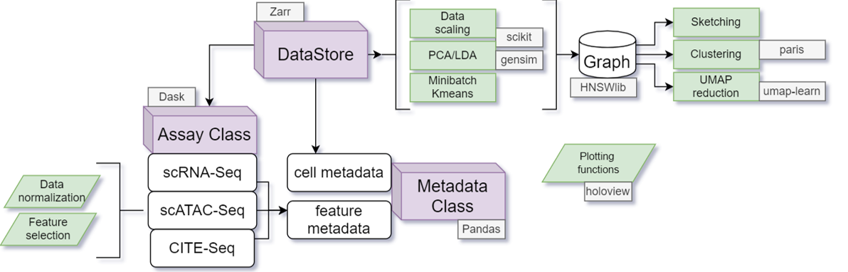
The following figure shows how different Class structures are connected to each other and the methods they contain. The DataStore class is the primary class that allows users to access all the data and functions. In almost all scenarios the user has to directly interact only with the object of DataStore class’s methods. DataStore object is linked to the underlying Zarr file hierarchy on the disk. We provide more details in the later sections.

The individual assays (in non mulit-omics datasets there will be only one assay) are represented as objects of the Assay class. A subclass of Assay class is automatically chosen based on the type of data. For example, RNAassay is chosen for single-cell RNA-Seq while ATACassaysubclass is chosen for scATAC-Seq. Each Assay subclass contains its own normalization and feature selection methods.

The Metadata class acts like a DataFrame (it is not actually a Dataframe but collections of columns/arrays that are loaded from disk on demand) that contains information on either individual cells or features. The cell metadata can directly be accessed from DataStore but feature metdata has to be accessed by the Assay object (we show examples below).

The DataStore class contains mutiple methods that allow generation of the KNN-graph that can be loaded to perform downsampling (sketching), clustering (Paris/Leiden) and UMAP/tSNE embedding (please see the basic workflows for usage of these methods).

%load_ext autotime

import scarf
scarf.__version__

'0.28.9'

time: 1.09 s (started: 2024-01-24 15:47:59 +00:00)

We download the CITE-Seq dataset that we analyzed earlier

scarf.fetch_dataset(
    dataset_name='tenx_8K_pbmc_citeseq',
    save_path='scarf_datasets',
    as_zarr=True
)

time: 24.2 s (started: 2024-01-24 15:48:00 +00:00)

ds = scarf.DataStore(
    'scarf_datasets/tenx_8K_pbmc_citeseq/data.zarr',
    nthreads=4
)

time: 42.3 ms (started: 2024-01-24 15:48:24 +00:00)

1) Zarr trees#

Scarf uses Zarr format to store raw counts as dense, chunked matrices. The Zarr file is in fact a directory that organizes the data in form of a tree. The count matrices, cell and features attributes, and all the data is stored in this Zarr hierarchy. Some of the key benefits of using Zarr over other formats like HDF5 are:

Parallel read and write access
Availability of compression algorithms like LZ4 that provides very high compression and decompression speeds.
Automatic storage of intermediate and processed data

In Scarf, the data is always synchronized between hard disk and RAM and as such there is no need to save data manually or synchronize the

We can inspect how the data is organized within the Zarr file using show_zarr_tree method of the DataStore.

ds.show_zarr_tree(depth=1)

/
 ├── ADT
 ├── RNA
 ├── cellData
 └── integratedGraphs
time: 2.83 ms (started: 2024-01-24 15:48:24 +00:00)

By setting depth=1 we get a look of the top-levels in the Zarr hierarchy: ‘RNA’, ‘ADT’ and ‘cellData’. The top levels here are hence composed of two assays and the cellData level, which will be explained below. Scarf attempts to store most of the data on disk immediately after it is processed. Since, that data that we have loaded is already preprocessed, below we can see that the calculated cell attributes can now be found under the cellData level. The cell-wise statistics that were calculated using ‘RNA’ assay have ‘RNA’ preppended to the name of the column. Similarly the columns stating with ‘ADT’ were created using ‘ADT’ assay data.

ds.show_zarr_tree(start='cellData')

cellData
 ├── ADT_UMAP1 (7865,) float32
 ├── ADT_UMAP2 (7865,) float32
 ├── ADT_leiden_cluster (7865,) int64
 ├── ADT_nCounts (7865,) float64
 ├── ADT_nFeatures (7865,) float64
 ├── I (7865,) bool
 ├── RNA+ADT_UMAP1 (7865,) float32
 ├── RNA+ADT_UMAP2 (7865,) float32
 ├── RNA+ADT_leiden_cluster (7865,) int64
 ├── RNA_UMAP1 (7865,) float32
 ├── RNA_UMAP2 (7865,) float32
 ├── RNA_cluster (7865,) int64
 ├── RNA_leiden_cluster (7865,) int64
 ├── RNA_nCounts (7865,) float64
 ├── RNA_nFeatures (7865,) float64
 ├── RNA_percentMito (7865,) float64
 ├── RNA_percentRibo (7865,) float64
 ├── RNA_tSNE1 (7865,) float64
 ├── RNA_tSNE2 (7865,) float64
 ├── ids (7865,) <U18
 └── names (7865,) <U18
time: 4.55 ms (started: 2024-01-24 15:48:24 +00:00)

The I column : This column is used to keep track of valid and invalid cells. The values in this column are boolean indicating which cells where filtered out (hence False) during filtering process. One of can think of column I as the default subset of cells that will be used for analysis if any other subset is not specifially chosen explicitly by the users. Most methods of DataStore object accept a parameter called cell_key and the default value for this paramter is I, which means that only cells with True in I column will be used.

If we inspect one of the assay, we will see the following zarr groups. The raw data matrix is stored under counts group (more on it in the next section). featureData is the feature level equivalent of cellData. featureData is explained in further detail in the next section. The markers level will be explained further in the last section. summary_stats_I contains statistics about features. These statistics are generally created during feature selection step. ‘normed__I__hvgs’ is explained in detail in the fourth section of this documentation.

ds.show_zarr_tree(start='RNA', depth=1)

RNA
 ├── counts (7865, 33538) uint32
 ├── featureData
 ├── markers
 ├── normed__I__hvgs
 └── summary_stats_I
time: 3.31 ms (started: 2024-01-24 15:48:24 +00:00)

The feature wise attributes for each assay are stored under the assays featureData level. The output below shows some of the feature level statistics.

ds.show_zarr_tree(start='RNA/featureData', depth=1)

featureData
 ├── I (33538,) bool
 ├── I__hvgs (33538,) bool
 ├── dropOuts (33538,) int64
 ├── ids (33538,) <U15
 ├── nCells (33538,) int64
 └── names (33538,) <U16
time: 3.15 ms (started: 2024-01-24 15:48:24 +00:00)

2) Cell and feature attributes#

The cell and feature level attributes can be accessed through DataStore, for example, using ds.cells and ds.RNA.feats respectively (both are objects of Metadata class). In this section we dive deeper into these attribute tables and try to perform CRUD operations on them.

head provides a quick look at the attribute tables.

ds.cells.head()

	I	ids	names	ADT_UMAP1	ADT_UMAP2	ADT_leiden_cluster	ADT_nCounts	ADT_nFeatures	RNA+ADT_UMAP1	RNA+ADT_UMAP2	...	RNA_UMAP1	RNA_UMAP2	RNA_cluster	RNA_leiden_cluster	RNA_nCounts	RNA_nFeatures	RNA_percentMito	RNA_percentRibo	RNA_tSNE1	RNA_tSNE2
0	True	AAACCCAAGATTGTGA-1	AAACCCAAGATTGTGA-1	-13.884989	9.510007	16	981.0	17.0	29.237206	20.219982	...	29.421942	-7.417822	4	3	6160.0	2194.0	8.668831	15.259740	-4.26865	-18.08830
1	True	AAACCCACATCGGTTA-1	AAACCCACATCGGTTA-1	-5.097915	10.784672	15	1475.0	17.0	32.570023	17.852776	...	30.801842	-12.649998	4	3	6713.0	2093.0	6.316103	19.037688	5.02671	-14.88920
2	True	AAACCCAGTACCGCGT-1	AAACCCAGTACCGCGT-1	-7.885502	12.961405	9	7149.0	17.0	25.061382	21.134617	...	29.397541	4.256729	5	5	3637.0	1518.0	8.056090	16.002200	-14.91320	-18.83030
3	True	AAACCCAGTATCGAAA-1	AAACCCAGTATCGAAA-1	12.072053	11.531997	2	6831.0	17.0	17.125492	-39.901890	...	5.441914	-32.227364	3	4	1244.0	737.0	9.003215	18.729904	16.69630	-3.35003
4	True	AAACCCAGTCGTCATA-1	AAACCCAGTCGTCATA-1	13.928782	12.290624	2	6839.0	17.0	17.794685	-40.299763	...	7.166490	-30.397615	3	4	2611.0	1240.0	6.204519	16.353887	18.37000	-1.37607

5 rows × 21 columns

time: 52.8 ms (started: 2024-01-24 15:48:24 +00:00)

The feature attribute table from any assay can similarly be quickly inspected

ds.RNA.feats.head()

	I	ids	names	I__hvgs	dropOuts	nCells
0	False	ENSG00000243485	MIR1302-2HG	False	7865	0
1	False	ENSG00000237613	FAM138A	False	7865	0
2	False	ENSG00000186092	OR4F5	False	7865	0
3	False	ENSG00000238009	AL627309.1	False	7853	12
4	False	ENSG00000239945	AL627309.3	False	7865	0

time: 18.9 ms (started: 2024-01-24 15:48:24 +00:00)

Even though the above ‘head’ command may make you think that ds.cells and ds.RNA.feats are Pandas dataframe, they in fact are not. If you wish to obtain a full table as Pandas dataframe, then you can export the columns of your choice as shown below.

ds.cells.to_pandas_dataframe(
    columns=['ids', 'RNA_UMAP1', 'RNA_UMAP2', 'RNA_cluster']
).set_index('ids')

	RNA_UMAP1	RNA_UMAP2	RNA_cluster
ids
AAACCCAAGATTGTGA-1	29.421942	-7.417822	4
AAACCCACATCGGTTA-1	30.801842	-12.649998	4
AAACCCAGTACCGCGT-1	29.397541	4.256729	5
AAACCCAGTATCGAAA-1	5.441914	-32.227364	3
AAACCCAGTCGTCATA-1	7.166490	-30.397615	3
...	...	...	...
TTTGTTGGTTCAAGTC-1	-5.545609	21.742104	18
TTTGTTGGTTGCATGT-1	-26.972895	-0.762715	9
TTTGTTGGTTGCGGCT-1	27.239552	-5.230516	4
TTTGTTGTCGAGTGAG-1	-23.030291	-20.647554	2
TTTGTTGTCGTTCAGA-1	-10.845096	-2.644977	2

7865 rows × 3 columns

time: 16.5 ms (started: 2024-01-24 15:48:24 +00:00)

If you wish to export all the columns as a dataframe then simply provide ds.cells.columns or ds.RNA.feats.columns as an argument rather than a list of columns. If you are interested in one of the columns then it can fetched using either fetch or fetch_all command.

fetch will provide values for a subset of cells (by default, only for those that have True value in column I, but any other boolean column can be given).

clusters = ds.cells.fetch('RNA_cluster')
clusters.shape

(7549,)

time: 5.6 ms (started: 2024-01-24 15:48:24 +00:00)

fetch_all will return values for all the cells.

clusters_all = ds.cells.fetch_all('RNA_cluster')
clusters_all.shape

(7865,)

time: 4.03 ms (started: 2024-01-24 15:48:24 +00:00)

If you wish to add a new column then insert command can be used for either cell or feature attributes. insert method will take care of inserting the values in the right rows even when a subset of values are provided. The default value for key parameter is I in insertmethod, so it will add values in same order as cells that have True value for I

is_clust_1 = clusters == 1   # is_clust_1 has just 7549 elements (same as the number of cells with value True in `I`)
ds.cells.insert(
    column_name='is_clust1', 
    values=is_clust_1
)

time: 5 ms (started: 2024-01-24 15:48:24 +00:00)

If we try to add values for a column that already exists then Scarf will throw an error. For example, if we simply rerun the command above, we should get an error

ds.cells.insert(
    column_name='is_clust1',
    values=is_clust_1
)

---------------------------------------------------------------------------
ValueError                                Traceback (most recent call last)
Cell In[14], line 1
----> 1 ds.cells.insert(
      2     column_name='is_clust1',
      3     values=is_clust_1
      4 )

File ~/checkouts/readthedocs.org/user_builds/scarf/envs/latest/lib/python3.10/site-packages/scarf/metadata.py:418, in MetaData.insert(self, column_name, values, fill_value, key, overwrite, location, force)
    414     raise ValueError(
    415         f"ERROR: {col} is a protected column name in MetaData class."
    416     )
    417 if col in self.columns and overwrite is False:
--> 418     raise ValueError(
    419         f"ERROR: {col} already exists. Please set `overwrite` to True to overwrite."
    420     )
    421 if isinstance(values, list):
    422     logger.debug(
    423         "'values' parameter is of `list` type and not `np.ndarray` as expected. The correct dtype "
    424         "may not be assigned to the column"
    425     )

ValueError: ERROR: is_clust1 already exists. Please set `overwrite` to True to overwrite.

time: 535 ms (started: 2024-01-24 15:48:24 +00:00)

To override this behaviour, you can use ‘overwrite’ parameter and set it to True

ds.cells.insert(
    column_name='is_clust1', 
    values=is_clust_1, 
    overwrite=True
)

time: 5.18 ms (started: 2024-01-24 15:48:25 +00:00)

Please checkout the API of the Metadata class to get information on how to perform other operations like delete and update columns.

3) Count matrices and data normalization#

Scarf uses Zarr format so that data can be stored in rectangular chunks. The raw data is saved in the counts level within each assay level in the Zarr hierarchy. It can easily be accessed as a Dask array using the rawData attribute of the assay. Note that for a standard analysis one would not interact with the raw data directly. Scarf internally optimizes the use of this Dask array to minimize the memory requirement of all operations.

ds.RNA.rawData

	Array	Chunk
Bytes	0.98 GiB	7.63 MiB
Shape	(7865, 33538)	(2000, 1000)
Dask graph	136 chunks in 1 graph layer
Data type	uint32 numpy.ndarray

time: 9.41 ms (started: 2024-01-24 15:48:25 +00:00)

The normalized data can be accessed through the normed method of the assay. In Scarf a user doesn’t need to perform normalization step manually, Scarf only stores the raw data and generates normalized data whenever needed. This means that Scarf may need to perform normalization several times. However, in practise we have noted that time spent in normalizing the data is only a small fraction of routine workflows.

ds.RNA.normed()

	Array	Chunk
Bytes	780.40 MiB	7.73 MiB
Shape	(7549, 13550)	(1934, 524)
Dask graph	136 chunks in 7 graph layers
Data type	float64 numpy.ndarray

time: 18.1 ms (started: 2024-01-24 15:48:25 +00:00)

Users can override how the normalization is performed in Scarf. Normalization is performed using the normMethod attribute which references the function responsible for performing the normalization.

ds.RNA.normMethod

<function scarf.assay.norm_lib_size(assay, counts: dask.array.core.Array) -> dask.array.core.Array>

time: 2.62 ms (started: 2024-01-24 15:48:25 +00:00)

Let’s checkout the source of function that is referenced by ds.RNA.normMethod

import inspect 

print (inspect.getsource(ds.RNA.normMethod))

def norm_lib_size(assay, counts: daskArrayType) -> daskArrayType:
    """Performs library size normalization on the data. This is the default
    method for RNA assays.

    Args:
        assay: An instance of the assay object
        counts: A dask array with raw counts data

    Returns:  A dask array (delayed matrix) containing normalized data.
    """
    return assay.sf * counts / assay.scalar.reshape(-1, 1)

time: 4.52 ms (started: 2024-01-24 15:48:25 +00:00)

Following is an example of how one can override the method of normalization

def my_cool_normalization_method(assay, counts):
    import numpy as np

    # Calculate total counts for each cell
    lib_size = counts.sum(axis=1).reshape(-1, 1) 
    
    # Library size normalization followed by log2 transformation
    return np.log2(counts/lib_size)

ds.RNA.normMethod = my_cool_normalization_method

time: 607 µs (started: 2024-01-24 15:48:25 +00:00)

Now whenever Scarf internally requires normalized values, this function will be used. Scarf provides a dummy normalization function (scarf.assay.norm_dummy) that does not perform normalization. This function can be useful if you have pre-normalized data and need to disable default normalization.

ds.RNA.normMethod = scarf.assay.norm_dummy

time: 347 µs (started: 2024-01-24 15:48:25 +00:00)

Please note: If you are using a custom function or disabling normalization, then everytime you load a DataStore object you will need to reassign normMethod to the function of your choice.

4) Data caching during graph creation#

All the results of make_graph step are saved under a name on the form ‘normed__{cell key}__{feature key}’ (placeholders used in brackets here). In this case, since we did not provide a cell key it takes default value of I, which means all the cells that were not filtered out. The feature key (feat_key) was set to hvgs. The Zarr directory is organized such that all the intermediate data is also saved. The intermediate data is organized in a hierarchy which triggers recomputation when upstream changes are detected. The parameter values are also saved in hierarchy level names. For example, ‘reduction_pca_31_I’ means that PCA linear dimension reduction with 31 PC axes was used and the PCA was fit across all the cells that have True value in column I.

ds.show_zarr_tree(start='RNA/normed__I__hvgs')

normed__I__hvgs
 ├── data (7549, 1995) float64
 ├── mu (997,) float64
 ├── reduction__pca__15__I
 │   ├── ann__l2__63__63__48__4466
 │   ├── kmeans__100__4466
 │   └── reduction (997, 15) float64
 ├── reduction__pca__30__I
 │   ├── ann__l2__63__63__48__4466
 │   ├── kmeans__100__4466
 │   ├── mu (1995,) float64
 │   ├── reduction (1995, 30) float64
 │   └── sigma (1995,) float64
 └── sigma (997,) float64
time: 5.81 ms (started: 2024-01-24 15:48:25 +00:00)

The graph calculated by make_graph can be easily loaded using the load_graph method, like below. The graph is loaded as a sparse matrix of the cells that were used for creating a graph.

Next, we show how the graph can be accessed if required. However, as stated above, normally Scarf handles the graph loading internally where required.

Because Scarf saves all the intermediate data, it might be the case that a lot of graphs are stored in the Zarr hierarchy. load_graph will load only the latest graph that was computed (for the given assay, cell key and feat key).

ds.load_graph(
    from_assay='RNA',
    cell_key='I',
    feat_key='hvgs',
    symmetric=False,
    upper_only=False
)

<7549x7549 sparse matrix of type '<class 'numpy.float64'>'
	with 158529 stored elements in Compressed Sparse Row format>

time: 17.9 ms (started: 2024-01-24 15:48:25 +00:00)

The sparse matrix above will load the If you would like to load a graph generated using some other parameter, then simply run make_graph again using those parameters. make_graph will not recalculate the graph if it already exists and will simply set it as the latest graph. This graph can then be loaded using load_graph

5) Fetching marker features#

Marker features (ex. marker genes) for a selection of cells can be calculated using run_marker_search. The markers for each group are stored under ‘marker’ group under the assay’s group. Within the ‘{assay}/markers’ level there are sublevels (only 1 here) created based on which cell set and cell groups were used: {cell_key}__{group_key}. Stored below this Zarr level are the individual group labels that contain the maker feature ids and their corresponding scores.

ds.show_zarr_tree(
    start='RNA/markers',
    depth=2
)

markers
 └── I__RNA_cluster
     ├── 1
     ├── 10
     ├── 11
     ├── 12
     ├── 13
     ├── 14
     ├── 15
     ├── 16
     ├── 17
     ├── 18
     ├── 19
     ├── 2
     ├── 20
     ├── 3
     ├── 4
     ├── 5
     ├── 6
     ├── 7
     ├── 8
     └── 9
time: 7.61 ms (started: 2024-01-24 15:48:25 +00:00)

Marker list for any group (e.x. cell cluster) can be fetched like below

ds.get_markers(
    group_key='RNA_cluster',
    group_id=7,
    min_score=0.1,
    min_frac_exp=0.1
)

	group_id	feature_name	feature_index	score	mean	mean_rest	frac_exp	frac_exp_rest	fold_change
0	7	KLRB1	20318.0	0.29927	14.13947	0.85409	0.98158	0.18971	16.55494
1	7	GZMK	8905.0	0.18346	5.50526	0.52044	0.98421	0.10852	10.57819
2	7	IL7R	8782.0	0.14324	7.44737	2.40312	0.97895	0.43186	3.09904
3	7	DUSP2	4135.0	0.13970	4.54737	0.68726	0.88947	0.29739	6.61662
4	7	NCR3	10623.0	0.10281	1.66053	0.19529	0.74737	0.13544	8.50308
5	7	KLRG1	20310.0	0.10096	1.72632	0.24578	0.79737	0.15274	7.02381

time: 250 ms (started: 2024-01-24 15:48:25 +00:00)

One can also export the names of markers for all the groups to a CSV file like below:

ds.export_markers_to_csv(
    group_key='RNA_cluster',
    csv_filename='test.csv',
    min_score=0.2,
    min_frac_exp=0.1
)

time: 4.93 s (started: 2024-01-24 15:48:25 +00:00)

That is all for this vignette.

Understanding how data is organized in Scarf

Sections