Estimating pseudotime ordering and expression dynamics#
%load_ext autotime

import scarf

scarf.__version__
'0.31.4'
time: 815 ms (started: 2025-04-15 15:43:59 +00:00)
1) Fetch pre-analyzed data#
Here we use the data from Bastidas-Ponce et al., 2019 Development for E15.5 stage of differentiation of endocrine cells from a pool of endocrine progenitors-precursors.
We have stored this data on Scarf’s online repository for quick access. We processed the data to identify the highly variable genes (top 2000) and create a neighbourhood graph of cells. A UMAP embedding was calculated for the cells.
scarf.fetch_dataset(
    dataset_name='bastidas-ponce_4K_pancreas-d15_rnaseq',
    save_path='./scarf_datasets',
    as_zarr=True,
)
time: 23 s (started: 2025-04-15 15:44:00 +00:00)
ds = scarf.DataStore(
    f"scarf_datasets/bastidas-ponce_4K_pancreas-d15_rnaseq/data.zarr",
    nthreads=4,
    default_assay='RNA'
)
time: 22.4 ms (started: 2025-04-15 15:44:23 +00:00)
ds
DataStore has 3413 (3696) cells with 1 assays: RNA
   Cell metadata:
            'I', 'ids', 'names', 'G2M_score', 'RNA_G2M_score',
            'RNA_S_score', 'RNA_UMAP1', 'RNA_UMAP2', 'RNA_cell_cycle_phase', 'RNA_cluster',
            'RNA_nCounts', 'RNA_nFeatures', 'RNA_percentMito', 'RNA_percentRibo', 'S_score',
            'clusters', 'clusters_coarse'
   RNA assay has 12497 (27998) features and following metadata:
            'I', 'ids', 'names', 'I__hvgs', 'dropOuts',
            'highly_variable_genes', 'nCells'
time: 4.92 ms (started: 2025-04-15 15:44:23 +00:00)
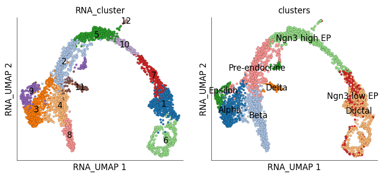
ds.plot_layout(
    layout_key='RNA_UMAP',
    color_by=['RNA_cluster', 'clusters'],
    width=4,
    height=4,
    legend_onside=False,
    cmap='tab20'
)
/home/docs/checkouts/readthedocs.org/user_builds/scarf/envs/latest/lib/python3.11/site-packages/scarf/plots.py:597: FutureWarning: The default of observed=False is deprecated and will be changed to True in a future version of pandas. Pass observed=False to retain current behavior or observed=True to adopt the future default and silence this warning.
  centers = df[[x, y, vc]].groupby(vc).median().T
time: 910 ms (started: 2025-04-15 15:44:23 +00:00)
2) Estimate pseudotime ordering#
In Scarf we use a memory efficient implementation of PBA algorithm (Weinreb et al. 2018, PNAS) to estimate a pseudotime ordering of cells. The function run_pseudotime_ordering can be run on any Assay for which we have calculated a neighbourhood graph. The the pseudotime is estimated in a supervised manner and hence, the user needs to provide the source (stem/progenitor/precursor cells) and sink (differentiated cell states) cell clusters/groups.
ds.run_pseudotime_scoring(
    source_sink_key="RNA_cluster",    # Column that contains cluster information
    sources=[1],                      # Source clusters
    sinks=[3],                        # Sink clusters
)
INFO: Calculating SVD of graph laplacian. This might take a while...
time: 1.39 s (started: 2025-04-15 15:44:24 +00:00)
By default, the calculated pseudotime values are saved under the cell attribute column ‘RNA_pseudotime’, where ‘RNA’ can be replaced by whatwever the name of the given assay is. Let’s visualize these values on UMAP plot. The lighter color cells represent beginning of the pseudotime
ds.plot_layout(
    layout_key='RNA_UMAP',
    color_by='RNA_pseudotime',
)

time: 223 ms (started: 2025-04-15 15:44:25 +00:00)
4) Visualize pseudotime correlated features#
In this section will do deeper on how to use the pseudotime correlation values for further exploratory analysis.
The first step is to export the values in a convenient dataframe format. we can use the to_pandas_dataframe methods of the feature attribute table to export the dataframe containing only the columns of choice
corr_genes_df = ds.RNA.feats.to_pandas_dataframe(
    columns=[
        'names',
        'I__RNA_pseudotime__p',
        'I__RNA_pseudotime__r'
    ],
    key='I')

# Rename the columns to be shorter
corr_genes_df.columns = ['names', 'p_value', 'r_value']
time: 8.86 ms (started: 2025-04-15 15:44:33 +00:00)
Let’s checkout the genes that are negatively correlated with the pseudotime. These genes increase in expression as the pseudotime progresses., i.e. as cells divide
corr_genes_df.sort_values('r_value')[:15]
| names | p_value | r_value | |
|---|---|---|---|
| 18864 | Spp1 | 0.0 | -0.853747 |
| 22385 | Rps19 | 0.0 | -0.811618 |
| 24581 | Rpl13 | 0.0 | -0.808717 |
| 431 | Dbi | 0.0 | -0.801796 |
| 16254 | Rps8 | 0.0 | -0.787065 |
| 19815 | Rpl32 | 0.0 | -0.777364 |
| 3163 | Sparc | 0.0 | -0.775107 |
| 26498 | Rps4x | 0.0 | -0.768438 |
| 20787 | Mgst1 | 0.0 | -0.762069 |
| 13425 | Rpl12 | 0.0 | -0.754217 |
| 25737 | Anxa2 | 0.0 | -0.751015 |
| 6983 | 1700011H14Rik | 0.0 | -0.745354 |
| 19142 | Cldn3 | 0.0 | -0.741470 |
| 10164 | Rps2 | 0.0 | -0.739792 |
| 8032 | Rpl3 | 0.0 | -0.736042 |
time: 5.33 ms (started: 2025-04-15 15:44:33 +00:00)
Let’s visualize the expression of some of these genes on the UMAP plot
ds.plot_layout(
    layout_key='RNA_UMAP',
    color_by=['Spp1', 'Dbi', 'Sparc'],
    width=3.5,
    height=3.5,
    point_size=5,
)

time: 748 ms (started: 2025-04-15 15:44:33 +00:00)
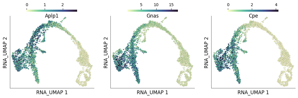
Now let’s checkout the genes that are most positively correlated with the pseudotime. These genes decrease in expression as the pseudotime progresses
corr_genes_df.sort_values('r_value', ascending=False)[:10]
| names | p_value | r_value | |
|---|---|---|---|
| 21244 | Aplp1 | 0.000000e+00 | 0.717088 |
| 14296 | Gnas | 0.000000e+00 | 0.708386 |
| 23549 | Cpe | 0.000000e+00 | 0.703213 |
| 3186 | Fam183b | 0.000000e+00 | 0.642701 |
| 25060 | Hmgn3 | 0.000000e+00 | 0.614297 |
| 26573 | Bex2 | 0.000000e+00 | 0.608843 |
| 8171 | Tuba1a | 0.000000e+00 | 0.594564 |
| 26730 | Pcsk1n | 0.000000e+00 | 0.593595 |
| 4284 | Ubb | 1.342275e-303 | 0.578068 |
| 2189 | Rap1b | 6.955857e-291 | 0.568015 |
time: 6.03 ms (started: 2025-04-15 15:44:34 +00:00)
ds.plot_layout(
    layout_key='RNA_UMAP',
    color_by=['Aplp1', 'Gnas', 'Cpe'],
    width=3.5,
    height=3.5,
    point_size=5,
)
time: 824 ms (started: 2025-04-15 15:44:34 +00:00)
5) Identify feature modules based on pseudotime#
run_pseudotime_marker_search is excellent to find the genes are linearly correlated with the pseudotime. This function provides us informative statistical metrics to identify genes that are most strongly correlated with the pseudotime. However, with these methods we do not recover all the dynamic patterns of expression along the pseudotime. For example, there might be certain genes that express only in the middle of the trajectory or in one branch of the trajectory.
run_pseudotime_aggregation performs two task: 1) It arranges cells along the pseudotime and creates a smoothened, scaled and binned matrix of data 2) Clustering (KNN+Paris) is performed on this matrix to identify the groups of features/genes that have similar expression patterns along the pseudotime.
ds.run_pseudotime_aggregation(
    pseudotime_key='RNA_pseudotime',
    cluster_label='pseudotime_clusters',
    n_clusters = 15,
    window_size=200,
    chunk_size=100,
)
INFO: Performing clustering, this might take a while...
time: 15.3 s (started: 2025-04-15 15:44:34 +00:00)
There are two primary results of run_pseudotime_aggregation:
The binned matrix is saved under
aggregate_<cell_key>_<feat_key>_<pseudotime_key>Feature clusters are saved under feature attributes table
# The binned data matrix. Here we print the shape of the matrix indicating the number of features and numner of bins respectively
ds.z.RNA.aggregated_I_I_RNA_pseudotime.data.shape
(12497, 100)
time: 2.39 ms (started: 2025-04-15 15:44:50 +00:00)
# Fetching pseudotime based cluster identity of features
ds.RNA.feats.fetch('pseudotime_clusters')
array([ 3, 12, 5, ..., 7, 7, 7])
time: 3.33 ms (started: 2025-04-15 15:44:50 +00:00)
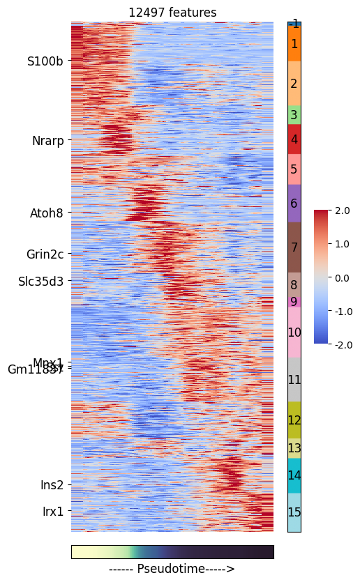
plot_pseudotime_heatmap allows visualizing the binned matrix along with the feature clusters
# Highlighting some marker genes
genes_to_label = ['S100b', 'Nrarp', 'Atoh8', 'Grin2c', 'Slc35d3',
                  'Sst', 'Mnx1', 'Ins2', 'Gm11837', 'Irx1']

ds.plot_pseudotime_heatmap(
    cell_key='I',
    feat_key='I',
    feature_cluster_key='pseudotime_clusters',
    pseudotime_key='RNA_pseudotime',
    show_features=genes_to_label
)
time: 1.05 s (started: 2025-04-15 15:44:50 +00:00)
The heatmap above shows the gene expression dynamics as the cells progress throught the pseudotime. Here, cluster 1 captures the genes that have highest expression in early pseudotime while cluster 15 captures genes whose expression peak in the late pseudotime.
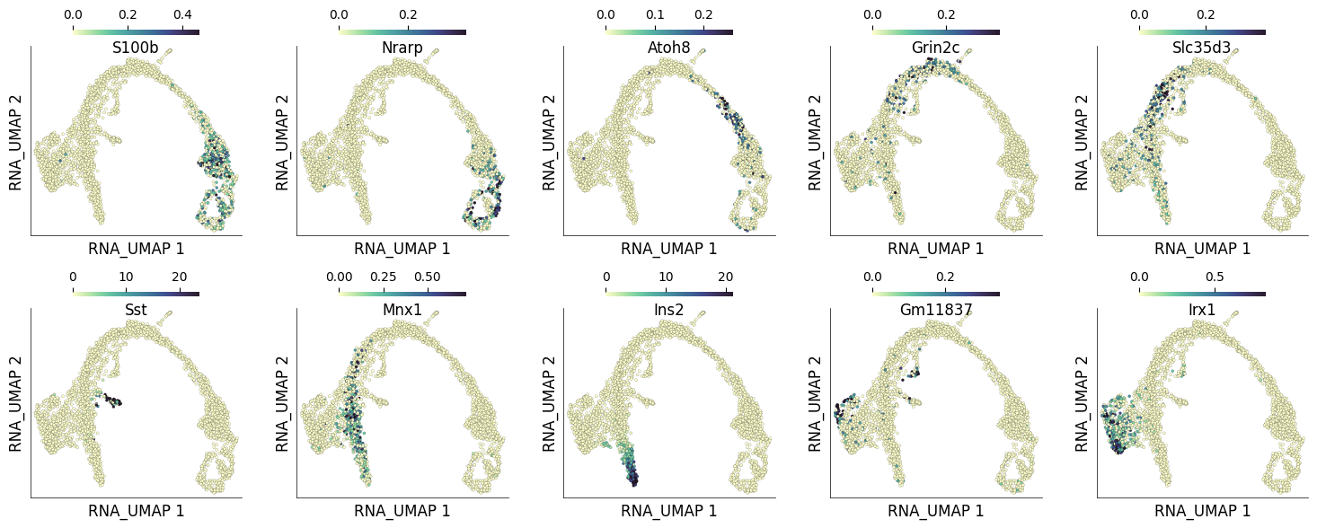
We can visualize the expression of the above selected genes on UMAP to check whether their cluster identity corroborates their expression pattern.
ds.plot_layout(
    layout_key='RNA_UMAP',
    color_by=genes_to_label,
    width=3,
    height=3,
    point_size=5,
    n_columns=5,
)
time: 2.34 s (started: 2025-04-15 15:44:51 +00:00)
6) Merging pseudotime-based feature modules into a new assay#
The pseudotime based clusters of features can be used create a new assay. add_grouped_assay will take each cluster and take the mean expression of genes from that cluster and add it to a new assay. The motivation behind this approach is that we do not have to add many columns to our cell metadata table and have the mean cluster values readily available for analysis.
Taking mean cluster values is a powerful approach that allows use to explore cumulative pattern of highly correlated genes. Here we create a new assay under title PTIME_MODULES
ds.add_grouped_assay(
    group_key='pseudotime_clusters',
    assay_label='PTIME_MODULES'
)
time: 5.1 s (started: 2025-04-15 15:44:53 +00:00)
# DataStore summary showing `PTIME_MODULES` assay with 15 features (number of pseudotime based feature clusters)
ds
DataStore has 3413 (3696) cells with 2 assays: PTIME_MODULES RNA
   Cell metadata:
            'I', 'ids', 'names', 'G2M_score', 'PTIME_MODULES_nCounts',
            'PTIME_MODULES_nFeatures', 'RNA_G2M_score', 'RNA_S_score', 'RNA_UMAP1', 'RNA_UMAP2',
            'RNA_cell_cycle_phase', 'RNA_cluster', 'RNA_nCounts', 'RNA_nFeatures', 'RNA_percentMito',
            'RNA_percentRibo', 'RNA_pseudotime', 'S_score', 'clusters', 'clusters_coarse',

   PTIME_MODULES assay has 15 (15) features and following metadata:
            'I', 'ids', 'names', 'dropOuts', 'nCells',

   RNA assay has 12497 (27998) features and following metadata:
            'I', 'ids', 'names', 'I__RNA_pseudotime__p', 'I__RNA_pseudotime__r',
            'I__hvgs', 'dropOuts', 'highly_variable_genes', 'nCells', 'pseudotime_clusters',
time: 6.73 ms (started: 2025-04-15 15:44:58 +00:00)
The mean values from each cluster are saved within the assay and tagged with names like group_1, group_2, etc
ds.PTIME_MODULES.feats.head()
| I | ids | names | dropOuts | nCells | |
|---|---|---|---|---|---|
| 0 | True | group_1 | group_1 | 0 | 3696 |
| 1 | True | group_2 | group_2 | 0 | 3696 |
| 2 | True | group_3 | group_3 | 0 | 3696 |
| 3 | True | group_4 | group_4 | 0 | 3696 |
| 4 | True | group_5 | group_5 | 0 | 3696 |
time: 10.9 ms (started: 2025-04-15 15:44:58 +00:00)
We can visualize these cluster mean values directly on the UMAP like this:
n_clusters = 15
ds.plot_layout(
    from_assay='PTIME_MODULES',
    layout_key='RNA_UMAP',
    color_by=[f"group_{i}" for i in range(1,n_clusters+1)],
    width=3,
    height=3,
    point_size=5,
    n_columns=5,
    cmap='coolwarm',
)

time: 2.92 s (started: 2025-04-15 15:44:58 +00:00)
This figure complements the heatmap we generated earlier very nicely. Using this approach we have clearly found gene modules that are restricted in expression to certain portion of the pseudotime and differentiation trajectory
7) Comparing pseudotime based feature modules with cluster markers#
Here we will compare the pseudotime based feature module extraction approach with classical cluster marker approach.
# Running marker search
ds.run_marker_search(group_key='RNA_cluster')
time: 8.39 s (started: 2025-04-15 15:45:01 +00:00)
Here we extract features from pseudotime-based cluster/group 13. These genes are the ones that show high expressio in Beta cells.
ptime_feat_clusts = ds.RNA.feats.to_pandas_dataframe(
    columns=['names', 'pseudotime_clusters']
)
ptime_based_markers = ptime_feat_clusts.names[ptime_feat_clusts.pseudotime_clusters == 13]
ptime_based_markers.head()
16      Tcf24
124     Mfsd9
260    Zfp142
274    Tuba4a
310    Trip12
Name: names, dtype: object
time: 9.37 ms (started: 2025-04-15 15:45:10 +00:00)
Now we extract all the marker genes for cell cluster 8, this cluster predominantly contains the Beta cells.
cell_cluster_markers = ds.get_markers(
    group_key='RNA_cluster',
    group_id='8'
).feature_name

cell_cluster_markers.head()
0        Ins2
1         Npy
2       Sytl4
3    Arhgap36
4     Tmem215
Name: feature_name, dtype: object
time: 145 ms (started: 2025-04-15 15:45:10 +00:00)
# let's checkout the number of Beta cell associated genes from both methods
ptime_based_markers.shape, cell_cluster_markers.shape
((486,), (90,))
time: 1.67 ms (started: 2025-04-15 15:45:10 +00:00)
# let's checkout the number of common Beta cell associated genes from both methods
len(set(cell_cluster_markers.index).intersection(ptime_based_markers.index))
1
time: 1.51 ms (started: 2025-04-15 15:45:10 +00:00)
Let’s visualize the cumulative expression of genes that are present only in cluster marker based approach
temp = list(set(cell_cluster_markers.index).difference(ptime_based_markers.index))
ds.cells.insert(
    column_name='Cell cluster based markers',
    values=ds.RNA.normed(feat_idx=sorted(temp)).mean(axis=1).compute(),
    overwrite=True)

ds.plot_layout(
    layout_key='RNA_UMAP',
    color_by='Cell cluster based markers',
    width=4, height=4, point_size=5, n_columns=5, cmap='coolwarm',
)

time: 230 ms (started: 2025-04-15 15:45:10 +00:00)
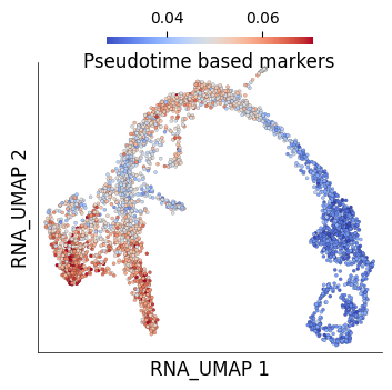
Let’s now do this the other way and visualize the cumulative expression of genes that are present only in pseudotime-based approach
temp = list(set(ptime_based_markers.index).difference(cell_cluster_markers.index))
ds.cells.insert(
    column_name='Pseudotime based markers',
    values=ds.RNA.normed(feat_idx=sorted(temp)).mean(axis=1).compute(),
    overwrite=True)

ds.plot_layout(
    layout_key='RNA_UMAP',
    color_by='Pseudotime based markers',
    width=4, height=4, point_size=5, n_columns=5, cmap='coolwarm',
)
time: 493 ms (started: 2025-04-15 15:45:10 +00:00)
The pseudotime-based approach clearly captures a lot of signal that would be otherwise missed by simply taking a cell cluster marker based approach.
That is all for this vignette.