Workflow for scATAC-Seq data#

If you haven’t already then we highly recommend that you please go the Workflow for scRNA-Seq analysis and also go through this vignette describing data organization and design principles of Scarf.

Here we will go through some of the basic steps of analysis of single-cell ATAC-seq (Assay for Transposase-Accessible Chromatin using sequencing) data.

%load_ext autotime

import scarf
scarf.__version__

'0.31.4'

time: 814 ms (started: 2025-04-15 15:22:20 +00:00)

1) Fetch and convert data#

We will use 10x Genomics’s singel-cell ATAC-Seq data from peripheral blood mononuclear cells. Like single-cell RNA-Seq, Scarf only needs a count matrix to start the analysis of scATAC-Seq data. We can use fetch_dataset to download the data in 10x’s HDF5 format.

scarf.fetch_dataset(
    dataset_name='tenx_10K_pbmc-v1_atacseq',
    save_path='scarf_datasets'
)

time: 23.4 s (started: 2025-04-15 15:22:20 +00:00)

The CrH5Reader class provides access to the HDF5 file. We can load the file and quickly check the number of features, and also verify that Scarf identified the assay as an ATAC assay.

reader = scarf.CrH5Reader(
    'scarf_datasets/tenx_10K_pbmc-v1_atacseq/data.h5'
)
reader.assayFeats

	ATAC
type	Peaks
start	0
end	89796
nFeatures	89796

time: 43.3 ms (started: 2025-04-15 15:22:44 +00:00)

writer = scarf.CrToZarr(
    reader,
    zarr_loc=f'scarf_datasets/tenx_10K_pbmc-v1_atacseq/data.zarr',
    chunk_size=(1000, 2000)
)
writer.dump(batch_size=1000)

time: 7.69 s (started: 2025-04-15 15:22:44 +00:00)

2) Create DataStore and filter cells#

We load the Zarr file on using DataStore class. The obtained DataStore object will be our single point on interaction for rest of this analysis. When loaded, Scarf will automatically calculate the number of cells where each peak is present and number of peaks that are accessible in cell (nFeatures). Scarf will also calculate the total number of fragments/cut sites within each cell.

ds = scarf.DataStore(
    'scarf_datasets/tenx_10K_pbmc-v1_atacseq/data.zarr', 
    nthreads=4
)

time: 6.22 s (started: 2025-04-15 15:22:52 +00:00)

We will use auto_filter_cells method which automatically remove outliers from the data. To identify outliers we generate a normal distribution using sample mean and variance. Using this normal distribution Scarf estimates the values with probability less 0.01 (default value) on both ends of the distribution and flags them for removal.

ds.auto_filter_cells()

INFO: 247 cells flagged for filtering out using attribute ATAC_nCounts

INFO: 294 cells flagged for filtering out using attribute ATAC_nFeatures

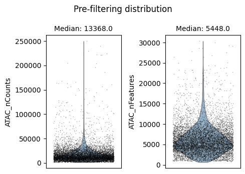
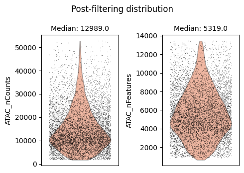
../_images/d50d44ff5ff5892f02bfabd1ba39d55a6a61818eda136732230090e57bbe37d4.png

../_images/c3e6a3cbbc1199f692d826364e3be28d1f76f1eebf25553915ad073fb80e28c1.png

time: 3.59 s (started: 2025-04-15 15:22:58 +00:00)

3) Feature selection#

For scATAC-Seq data, the features are ranked by their TF-IDF normalized values, summed across all cells. The top n features are marked as prevalent_peaks and are used for downstream steps. Here we used top 25000 peaks, which makes for more than quarter of all the peaks which inline with the what has been suggested in other scATAC-Seq analysis protocols.

ds.mark_prevalent_peaks(top_n=25000)

time: 5.37 s (started: 2025-04-15 15:23:01 +00:00)

ds.ATAC.feats.head()

	I	ids	names	I__prevalent_peaks	dropOuts	nCells	stats_I_prevalence
0	True	chr1:565107-565550	chr1:565107-565550	False	8645	83	0.206181
1	True	chr1:569174-569639	chr1:569174-569639	False	8529	199	0.350725
2	True	chr1:713460-714823	chr1:713460-714823	True	6242	2486	1.993573
3	True	chr1:752422-753038	chr1:752422-753038	True	8296	432	0.680701
4	True	chr1:762106-763359	chr1:762106-763359	True	6850	1878	1.570790

time: 20.5 ms (started: 2025-04-15 15:23:07 +00:00)

4) KNN graph creation#

For scATAC-Seq datasets, Scarf uses TF-IDF normalization. The normalization is automatically performed during the graph building step. The selected features, marked as prevalent_peaks in feature metadata, are used for graph creation. For the dimension reduction step, LSI (latent semantic indexing) is used rather than PCA. The rest of the steps are same as for scRNA-Seq data.

LSI reduction of scATAC-Seq is known to capture the sequencing depth of cells in the first LSI dimension. Hence, by default, the lsi_skip_first parameter is True but users can override it.

ds.make_graph(
    feat_key='prevalent_peaks',
    k=21,
    dims=50,
    n_centroids=100,
    lsi_skip_first=True,
)

---------------------------------------------------------------------------
KeyboardInterrupt                         Traceback (most recent call last)
Cell In[9], line 1
----> 1 ds.make_graph(
   feat_key='prevalent_peaks',
   k=21,
   dims=50,
   n_centroids=100,
   lsi_skip_first=True,
)

File ~/checkouts/readthedocs.org/user_builds/scarf/envs/latest/lib/python3.11/site-packages/scarf/datastore/graph_datastore.py:992, in GraphDataStore.make_graph(self, from_assay, cell_key, feat_key, pca_cell_key, reduction_method, dims, k, ann_metric, ann_efc, ann_ef, ann_m, ann_parallel, rand_state, n_centroids, batch_size, log_transform, renormalize_subset, local_connectivity, bandwidth, update_keys, return_ann_object, custom_loadings, feat_scaling, lsi_skip_first, harmonize, batch_columns, show_elbow_plot, ann_index_fetcher, ann_index_saver)
   recall = self_query_knn(
       ann_obj=ann_obj,
       store=self.zw.create_group(knn_loc, overwrite=True),
       chunk_size=batch_size,
       nthreads=self.nthreads,
   )
   recall = "%.2f" % recall
--> 992 smoothen_dists(
   self.zw.create_group(graph_loc, overwrite=True),
   self.zw[knn_loc]["indices"],
   self.zw[knn_loc]["distances"],
   local_connectivity,
   bandwidth,
   batch_size,
)
if recall is not None:
   logger.info(f"ANN recall: {recall}%")

File ~/checkouts/readthedocs.org/user_builds/scarf/envs/latest/lib/python3.11/site-packages/scarf/knn_utils.py:132, in smoothen_dists(store, z_idx, z_dist, lc, bw, chunk_size)
sigmas, rhos = smooth_knn_dist(
   kv, k=n_neighbors, local_connectivity=lc, bandwidth=bw
)
if umap_is_latest:
--> 132     rows, cols, vals, _ = compute_membership_strengths(ki, kv, sigmas, rhos)
else:
   rows, cols, vals = compute_membership_strengths(ki, kv, sigmas, rhos)

File ~/checkouts/readthedocs.org/user_builds/scarf/envs/latest/lib/python3.11/site-packages/numba/core/dispatcher.py:376, in _DispatcherBase._compile_for_args(self, *args, **kws)
return_val = None
try:
--> 376     return_val = self.compile(tuple(argtypes))
except errors.ForceLiteralArg as e:
   # Received request for compiler re-entry with the list of arguments
   # indicated by e.requested_args.
   # First, check if any of these args are already Literal-ized
   already_lit_pos = [i for i in e.requested_args
                      if isinstance(args[i], types.Literal)]

File ~/checkouts/readthedocs.org/user_builds/scarf/envs/latest/lib/python3.11/site-packages/numba/core/dispatcher.py:904, in Dispatcher.compile(self, sig)
with ev.trigger_event("numba:compile", data=ev_details):
   try:
--> 904         cres = self._compiler.compile(args, return_type)
   except errors.ForceLiteralArg as e:
       def folded(args, kws):

File ~/checkouts/readthedocs.org/user_builds/scarf/envs/latest/lib/python3.11/site-packages/numba/core/dispatcher.py:80, in _FunctionCompiler.compile(self, args, return_type)
def compile(self, args, return_type):
---> 80     status, retval = self._compile_cached(args, return_type)
   if status:
       return retval

File ~/checkouts/readthedocs.org/user_builds/scarf/envs/latest/lib/python3.11/site-packages/numba/core/dispatcher.py:94, in _FunctionCompiler._compile_cached(self, args, return_type)
   pass
try:
---> 94     retval = self._compile_core(args, return_type)
except errors.TypingError as e:
   self._failed_cache[key] = e

File ~/checkouts/readthedocs.org/user_builds/scarf/envs/latest/lib/python3.11/site-packages/numba/core/dispatcher.py:107, in _FunctionCompiler._compile_core(self, args, return_type)
flags = self._customize_flags(flags)
impl = self._get_implementation(args, {})
--> 107 cres = compiler.compile_extra(self.targetdescr.typing_context,
                             self.targetdescr.target_context,
                             impl,
                             args=args, return_type=return_type,
                             flags=flags, locals=self.locals,
                             pipeline_class=self.pipeline_class)
# Check typing error if object mode is used
if cres.typing_error is not None and not flags.enable_pyobject:

File ~/checkouts/readthedocs.org/user_builds/scarf/envs/latest/lib/python3.11/site-packages/numba/core/compiler.py:739, in compile_extra(typingctx, targetctx, func, args, return_type, flags, locals, library, pipeline_class)
"""Compiler entry point

Parameter
   (...)    735     compiler pipeline
"""
pipeline = pipeline_class(typingctx, targetctx, library,
                         args, return_type, flags, locals)
--> 739 return pipeline.compile_extra(func)

File ~/checkouts/readthedocs.org/user_builds/scarf/envs/latest/lib/python3.11/site-packages/numba/core/compiler.py:439, in CompilerBase.compile_extra(self, func)
self.state.lifted = ()
self.state.lifted_from = None
--> 439 return self._compile_bytecode()

File ~/checkouts/readthedocs.org/user_builds/scarf/envs/latest/lib/python3.11/site-packages/numba/core/compiler.py:505, in CompilerBase._compile_bytecode(self)
"""
Populate and run pipeline for bytecode input
"""
assert self.state.func_ir is None
--> 505 return self._compile_core()

File ~/checkouts/readthedocs.org/user_builds/scarf/envs/latest/lib/python3.11/site-packages/numba/core/compiler.py:473, in CompilerBase._compile_core(self)
res = None
try:
--> 473     pm.run(self.state)
   if self.state.cr is not None:
       break

File ~/checkouts/readthedocs.org/user_builds/scarf/envs/latest/lib/python3.11/site-packages/numba/core/compiler_machinery.py:356, in PassManager.run(self, state)
pass_inst = _pass_registry.get(pss).pass_inst
if isinstance(pass_inst, CompilerPass):
--> 356     self._runPass(idx, pass_inst, state)
else:
   raise BaseException("Legacy pass in use")

File ~/checkouts/readthedocs.org/user_builds/scarf/envs/latest/lib/python3.11/site-packages/numba/core/compiler_lock.py:35, in _CompilerLock.__call__.<locals>._acquire_compile_lock(*args, **kwargs)
@functools.wraps(func)
def _acquire_compile_lock(*args, **kwargs):
   with self:
---> 35         return func(*args, **kwargs)

File ~/checkouts/readthedocs.org/user_builds/scarf/envs/latest/lib/python3.11/site-packages/numba/core/compiler_machinery.py:311, in PassManager._runPass(self, index, pss, internal_state)
   mutated |= check(pss.run_initialization, internal_state)
with SimpleTimer() as pass_time:
--> 311     mutated |= check(pss.run_pass, internal_state)
with SimpleTimer() as finalize_time:
   mutated |= check(pss.run_finalizer, internal_state)

File ~/checkouts/readthedocs.org/user_builds/scarf/envs/latest/lib/python3.11/site-packages/numba/core/compiler_machinery.py:272, in PassManager._runPass.<locals>.check(func, compiler_state)
def check(func, compiler_state):
--> 272     mangled = func(compiler_state)
   if mangled not in (True, False):
       msg = ("CompilerPass implementations should return True/False. "
              "CompilerPass with name '%s' did not.")

File ~/checkouts/readthedocs.org/user_builds/scarf/envs/latest/lib/python3.11/site-packages/numba/core/typed_passes.py:112, in BaseTypeInference.run_pass(self, state)
"""
Type inference and legalization
"""
with fallback_context(state, 'Function "%s" failed type inference'
                     % (state.func_id.func_name,)):
   # Type inference
--> 112     typemap, return_type, calltypes, errs = type_inference_stage(
       state.typingctx,
       state.targetctx,
       state.func_ir,
       state.args,
       state.return_type,
       state.locals,
       raise_errors=self._raise_errors)
   state.typemap = typemap
   # save errors in case of partial typing

File ~/checkouts/readthedocs.org/user_builds/scarf/envs/latest/lib/python3.11/site-packages/numba/core/typed_passes.py:93, in type_inference_stage(typingctx, targetctx, interp, args, return_type, locals, raise_errors)
   infer.build_constraint()
   # return errors in case of partial typing
---> 93     errs = infer.propagate(raise_errors=raise_errors)
   typemap, restype, calltypes = infer.unify(raise_errors=raise_errors)
return _TypingResults(typemap, restype, calltypes, errs)

File ~/checkouts/readthedocs.org/user_builds/scarf/envs/latest/lib/python3.11/site-packages/numba/core/typeinfer.py:1066, in TypeInferer.propagate(self, raise_errors)
oldtoken = newtoken
# Errors can appear when the type set is incomplete; only
# raise them when there is no progress anymore.
-> 1066 errors = self.constraints.propagate(self)
newtoken = self.get_state_token()
self.debug.propagate_finished()

File ~/checkouts/readthedocs.org/user_builds/scarf/envs/latest/lib/python3.11/site-packages/numba/core/typeinfer.py:160, in ConstraintNetwork.propagate(self, typeinfer)
with typeinfer.warnings.catch_warnings(filename=loc.filename,
                                      lineno=loc.line):
   try:
--> 160         constraint(typeinfer)
   except ForceLiteralArg as e:
       errors.append(e)

File ~/checkouts/readthedocs.org/user_builds/scarf/envs/latest/lib/python3.11/site-packages/numba/core/typeinfer.py:692, in IntrinsicCallConstraint.__call__(self, typeinfer)
if fnty in utils.OPERATORS_TO_BUILTINS:
   fnty = typeinfer.resolve_value_type(None, fnty)
--> 692 self.resolve(typeinfer, typeinfer.typevars, fnty=fnty)

File ~/checkouts/readthedocs.org/user_builds/scarf/envs/latest/lib/python3.11/site-packages/numba/core/typeinfer.py:589, in CallConstraint.resolve(self, typeinfer, typevars, fnty)
   fnty = fnty.instance_type
try:
--> 589     sig = typeinfer.resolve_call(fnty, pos_args, kw_args)
except ForceLiteralArg as e:
   # Adjust for bound methods
   folding_args = ((fnty.this,) + tuple(self.args)
                   if isinstance(fnty, types.BoundFunction)
                   else self.args)

File ~/checkouts/readthedocs.org/user_builds/scarf/envs/latest/lib/python3.11/site-packages/numba/core/typeinfer.py:1560, in TypeInferer.resolve_call(self, fnty, pos_args, kw_args)
   return sig
else:
   # Normal non-recursive call
-> 1560     return self.context.resolve_function_type(fnty, pos_args, kw_args)

File ~/checkouts/readthedocs.org/user_builds/scarf/envs/latest/lib/python3.11/site-packages/numba/core/typing/context.py:195, in BaseContext.resolve_function_type(self, func, args, kws)
# Prefer user definition first
try:
--> 195     res = self._resolve_user_function_type(func, args, kws)
except errors.TypingError as e:
   # Capture any typing error
   last_exception = e

File ~/checkouts/readthedocs.org/user_builds/scarf/envs/latest/lib/python3.11/site-packages/numba/core/typing/context.py:247, in BaseContext._resolve_user_function_type(self, func, args, kws, literals)
       return self.resolve_function_type(func_type, args, kws)
if isinstance(func, types.Callable):
   # XXX fold this into the __call__ attribute logic?
--> 247     return func.get_call_type(self, args, kws)

File ~/checkouts/readthedocs.org/user_builds/scarf/envs/latest/lib/python3.11/site-packages/numba/core/types/functions.py:308, in BaseFunction.get_call_type(self, context, args, kws)
       nolitargs = tuple([_unlit_non_poison(a) for a in args])
       nolitkws = {k: _unlit_non_poison(v)
                   for k, v in kws.items()}
--> 308         sig = temp.apply(nolitargs, nolitkws)
except Exception as e:
   if not isinstance(e, errors.NumbaError):

File ~/checkouts/readthedocs.org/user_builds/scarf/envs/latest/lib/python3.11/site-packages/numba/core/typing/templates.py:490, in ConcreteTemplate.apply(self, args, kws)
def apply(self, args, kws):
   cases = getattr(self, 'cases')
--> 490     return self._select(cases, args, kws)

File ~/checkouts/readthedocs.org/user_builds/scarf/envs/latest/lib/python3.11/site-packages/numba/core/typing/templates.py:284, in FunctionTemplate._select(self, cases, args, kws)
def _select(self, cases, args, kws):
   options = {
       'unsafe_casting': self.unsafe_casting,
       'exact_match_required': self.exact_match_required,
   }
--> 284     selected = self.context.resolve_overload(self.key, cases, args, kws,
                                            **options)
   return selected

File ~/checkouts/readthedocs.org/user_builds/scarf/envs/latest/lib/python3.11/site-packages/numba/core/typing/context.py:635, in BaseContext.resolve_overload(self, key, cases, args, kws, allow_ambiguous, unsafe_casting, exact_match_required)
for case in cases:
   if len(args) == len(case.args):
--> 635         rating = self._rate_arguments(args, case.args, **options)
       if rating is not None:
           candidates.append((rating.astuple(), case))

File ~/checkouts/readthedocs.org/user_builds/scarf/envs/latest/lib/python3.11/site-packages/numba/core/typing/context.py:575, in BaseContext._rate_arguments(self, actualargs, formalargs, unsafe_casting, exact_match_required)
rate = Rating()
for actual, formal in zip(actualargs, formalargs):
--> 575     conv = self.can_convert(actual, formal)
   if conv is None:
       return None

File ~/checkouts/readthedocs.org/user_builds/scarf/envs/latest/lib/python3.11/site-packages/numba/core/typing/context.py:551, in BaseContext.can_convert(self, fromty, toty)
   return Conversion.exact
else:
   # First check with the type manager (some rules are registered
   # at startup there, see numba.typeconv.rules)
--> 551     conv = self.tm.check_compatible(fromty, toty)
   if conv is not None:
       return conv

File ~/checkouts/readthedocs.org/user_builds/scarf/envs/latest/lib/python3.11/site-packages/numba/core/typeconv/typeconv.py:44, in TypeManager.check_compatible(self, fromty, toty)
if not isinstance(toty, types.Type):
   raise ValueError("Specified type '%s' (%s) is not a Numba type" %
                    (toty, type(toty)))
---> 44 name = _typeconv.check_compatible(self._ptr, fromty._code, toty._code)
conv = Conversion[name] if name is not None else None
assert conv is not Conversion.nil

KeyboardInterrupt: 

time: 3min 21s (started: 2025-04-15 15:23:07 +00:00)

5) UMAP reduction and clustering#

Non-linear dimension reduction using UMAP and tSNE are performed in the same way as for scRNA-Seq data. Because, in Scarf the core UMAP step are run directly on the neighbourhood graph, the scATAC-Seq data is handled similar to any other data.

ds.run_umap(
    n_epochs=500,
    min_dist=0.1, 
    spread=1, 
    parallel=True
)

Same goes for clustering as well. The leiden clustering acts on the neighbourhood graph directly.

ds.run_leiden_clustering(resolution=0.6)

Results from both UMAP and Leiden clustering are stored in cell attribute table. Here, because the UMAP and leiden clustering columns have ‘ATAC’ prefixes because they were executed on the default ‘ATAC’ assay. You can also see that the cells that were filtered out (marked by ‘False’ value in column ‘I’) have NaN value for UMAP axes and -1 for clustering

ds.cells.head()

We can visualize the UMAP embedding and the clusters of cells on the embedding

ds.plot_layout(
    layout_key='ATAC_UMAP', 
    color_by='ATAC_leiden_cluster'
)

Those familiar with PBMC datasets might already be able to identify different cell types in the UMAP plot.

6) Calculating gene scores#

The features in snATAC-Seq in form of peak coordinates are hard to interpret by themselves. Hence, distilling the open chromatin regions in terms of accessible genes can help in identification of cell types. GeneScores are simply the summation of all the peak fragments that are present within gene bodies and their corresponding promoter region. Since, marker genes are often better understood than the non-coding regions the GeneScores can be used to annotate cell types.

In Scarf, the users can provide a BED file containing gene annotations. This BED should have no header, should be tab separated and must have the columns in following order:

chromosome identifier
start coordinate
end coordinate
Gene ID
Gene Name
Strand (Optional)

The start/end coordinate can extend through transcription start site (TSS) to include a portion of promoter.

For convenience we have generated such BED files for human and mouse assemblies using the annotation information from GENCODE project. We downloaded the GFF3 format primary chromosome annotations and used Scarf’s GFFReader to convert the files into BED and add promoter offset of 2KB. These BED files containing gene annotations can be downloaded using fetch_dataset command and passing ‘annotations’ parameter.

scarf.fetch_dataset(
    dataset_name='annotations', 
    save_path='scarf_datasets'
)

Now we have the annotations and are ready to calculate the ‘GeneScores’. The add_melded_assay is the DataStore method that will be used for this purpose. The add_melded_assay method is actually designed to map any arbitrary genomic coordinate information (not just gene annotations) to the ATAC peaks. Here, we use the term ‘melding’ for the process wherein for a given loci the values from all the overlapping peaks are merged/melded into that feature. The peaks values are TF-IDF normalized before melding.

Now we explain the parameters that are usually passed to the add_melded_assay.

from_assay: Name of the assay to be acted on. You can generally skip if you have only one assay. We use this parameter here only for demonstration puspose
external_bed_fn: This is the annotation file. Here we pass the annotation for human GRCh37/hg19 assembly based GENCODE v38 annotations.
peak_col: This is the column in ds.ATAC.feats table that contains the peak coordinates. In this case it is ‘ids’, but could be anyt other column. Please note that the coordinate information in this column should be in format ‘chr:start-end’ (please note the positions of colon and hyphen)
renormalization: By overriding the default value of True to False here, we turned off ‘renormalization’ step. The renormalization step makes sure that all the feature values for each cells in the melded assay sum up to the same value. Here we turned this off because we will have ‘GeneScores’ as an ‘RNAassay’ which uses library size normalization that has the same effect as ‘renormalization’.
assay_label: The label/name of the melded/output assay. Because we are using gene bodies as our input, ‘GeneScores’ is sensible choice.
assay_type: Here we set the type of assay as ‘RNA’ which means that the new melded assay will be treated as if it was an scRNA-Seq assay. Alternatively, we could have set it as a generic ‘Assay’

ds.add_melded_assay(
    from_assay='ATAC',
    external_bed_fn='scarf_datasets/annotations/human_GRCh37_gencode_v38_gene_body.bed.gz',
    peaks_col='ids',
    renormalization=False,
    assay_label='GeneScores',
    assay_type='RNA'
)

We can now print out the DataStore and see that the ‘GeneScores’ assay has indeed been added. The ‘add_melded_assay’ also printed a useful bit of information that almost half of features(genes bodies) did not overlap with even a single peak. The melded assay anyway contains all the genes but sets these ‘empty’ genes as invalid.

ds

Let’s now visualize some ‘GeneScores’ for some of the known marker genes for PBMCs on the UMAP plot calculated on the ATAC assay

ds.plot_layout(
    layout_key='ATAC_UMAP', from_assay='GeneScores', 
    color_by=['CD3D', 'MS4A1', 'LEF1', 'NKG7', 'TREM1', 'LYZ'],
    clip_fraction=0.01, 
    n_columns=3,
    width=3,
    height=3,
    point_size=5,
    scatter_kwargs={'lw': 0.01},
)

We stop here in this vignette. But will soon add other vignettes that show how we can other kinds of melded assays like motifs, enhancers, etc. We will also explore how we can use the ‘GeneScores’ to integrate scATAC-Seq datasets with scRNA-Seq datasets from same population of cells (but not the exact same set of cells)

That is all for this vignette.

Workflow for scATAC-Seq data

Sections