Cell subsampling using TopACeDo¶

[1]:

%load_ext autotime
%config InlineBackend.figure_format = 'retina'

import scarf
scarf.__version__

[1]:

'0.8.5'

time: 947 ms (started: 2021-08-22 18:39:24 +00:00)

1) Installing dependencies¶

We need to install the TopACeDo algorithm to perform subsampling:

[2]:

!pip install git+https://github.com/fraenkel-lab/pcst_fast.git@deb3236cc26ee9fee77d5af40fac3f12bb753850
!pip install -U topacedo

Collecting git+https://github.com/fraenkel-lab/pcst_fast.git@deb3236cc26ee9fee77d5af40fac3f12bb753850
  Cloning https://github.com/fraenkel-lab/pcst_fast.git (to revision deb3236cc26ee9fee77d5af40fac3f12bb753850) to /tmp/pip-req-build-wfjg_17i
  Running command git clone -q https://github.com/fraenkel-lab/pcst_fast.git /tmp/pip-req-build-wfjg_17i
  Running command git rev-parse -q --verify 'sha^deb3236cc26ee9fee77d5af40fac3f12bb753850'
  Running command git fetch -q https://github.com/fraenkel-lab/pcst_fast.git deb3236cc26ee9fee77d5af40fac3f12bb753850
  Running command git checkout -q deb3236cc26ee9fee77d5af40fac3f12bb753850
  Resolved https://github.com/fraenkel-lab/pcst_fast.git to commit deb3236cc26ee9fee77d5af40fac3f12bb753850
Requirement already satisfied: pybind11>=2.1.0 in /home/docs/checkouts/readthedocs.org/user_builds/scarf/envs/0.8.5/lib/python3.8/site-packages (from pcst-fast==1.0.7) (2.7.1)
Building wheels for collected packages: pcst-fast
  Building wheel for pcst-fast (setup.py) ... - \ | / - \ done
  Created wheel for pcst-fast: filename=pcst_fast-1.0.7-cp38-cp38-linux_x86_64.whl size=840719 sha256=cd4c11ec15f07d1366fcdbe207d1287ae15393742fd5ede48531b25613b665ac
  Stored in directory: /home/docs/.cache/pip/wheels/48/f1/74/6bb2e9cc262228dbdc63916ec60f0717574b5f633b6ee30b0a
Successfully built pcst-fast
Installing collected packages: pcst-fast
Successfully installed pcst-fast-1.0.7
Requirement already satisfied: topacedo in /home/docs/checkouts/readthedocs.org/user_builds/scarf/envs/0.8.5/lib/python3.8/site-packages (0.2.7)
time: 13.2 s (started: 2021-08-22 18:39:25 +00:00)

2) Fetching pre-processed data¶

[3]:

# Loading preanalyzed dataset that was processed in the `basic_tutorial` vignette
scarf.fetch_dataset('tenx_5K_pbmc_rnaseq', as_zarr=True, save_path='scarf_datasets')

INFO: Download started...
INFO: Download finished! File saved here: /home/docs/checkouts/readthedocs.org/user_builds/scarf/checkouts/0.8.5/docs/source/vignettes/scarf_datasets/tenx_5K_pbmc_rnaseq/data.zarr.tar.gz
INFO: Extracting Zarr file for tenx_5K_pbmc_rnaseq

2021-08-22 18:39:48 URL:https://storage.googleapis.com/cos-osf-prod-files-de-1/1ef8b465325d04f0b87ed06fe7813ec6698d1a9a45e3511e885ae45e732f9bb8?response-content-disposition=attachment%3B%20filename%3D%22data.zarr.tar.gz%22%3B%20filename%2A%3DUTF-8%27%27data.zarr.tar.gz&GoogleAccessId=files-de-1%40cos-osf-prod.iam.gserviceaccount.com&Expires=1629657646&Signature=cbvXg8qIy4XVn6FuHtZZrS450%2BaO6F2RUz%2BuvXZWTiUeyMdGCOgOm7TRmsLC6CsTq7thfXbF30NvgAGS0QGHTgOOIaB68fFKKA6iP5XFHTbjfbVFWkX568ZKeFULBXMNpM6obE27op2ILn1wRoGtaQegna7vNpD7v2wp8N%2BgTyMi2mkO9DZj%2FQisPDa5Q%2BUpEEAuOK%2Bbch75z2EhCH71s1fJfQWwMWCCzvenb3i7yKRWhezoiWw29xmyKbvpbnwvu0rPpY0KhnGQBB%2B1qkMWVtM2mqLZkqwHRDE5yjJGZm8MsGOIXG7zL4LE%2F%2BN4xZdaZKspiBvTl7eERSqHMH095g%3D%3D [31491651/31491651] -> "/home/docs/checkouts/readthedocs.org/user_builds/scarf/checkouts/0.8.5/docs/source/vignettes/scarf_datasets/tenx_5K_pbmc_rnaseq/data.zarr.tar.gz" [1]

time: 10 s (started: 2021-08-22 18:39:38 +00:00)

[4]:

ds = scarf.DataStore('scarf_datasets/tenx_5K_pbmc_rnaseq/data.zarr')
ds.plot_layout(layout_key='RNA_UMAP', color_by='RNA_cluster')

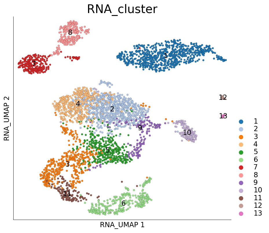
../_images/vignettes_cell_subsampling_tutorial_7_0.png

time: 1.06 s (started: 2021-08-22 18:39:48 +00:00)

3) Run TopACeDo downsampler¶

UMAP, clustering and marker identification together allow a good understanding of cellular diversity. However, one can still choose from a plethora of other analysis on the data. For example, identification of cell differentiation trajectories. One of the major challenges to run these analysis could be the size of the data. Scarf performs a topology conserving downsampling of the data based on the cell neighbourhood graph. This downsampling aims to maximize the heterogeneity while sampling cells from the data.

Here we run the TopACeDo downsampling algorithm that leverages Scarf’s KNN graph to perform a manifold preserving subsampling of cells. The subsampler can be invoked directly from Scarf’s DataStore object.

[5]:

ds.run_topacedo_sampler(cluster_key='RNA_cluster', max_sampling_rate=0.1)

Constructing graph from dendrogram: 100%|██████████| 3939/3939 [00:00<00:00, 56343.64it/s]

INFO: 384 cells (9.75%) sub-sampled. Subsample to Seed (165 cells) ratio: 2.327
INFO: Sketched cells saved under column 'RNA_sketched'
INFO: Cell neighbourhood densities saved under column: 'RNA_cell_density'
INFO: Mean SNN values saved under column: 'RNA_snn_value'
INFO: Seed cells saved under column: 'RNA_sketch_seeds'
time: 1.25 s (started: 2021-08-22 18:39:50 +00:00)

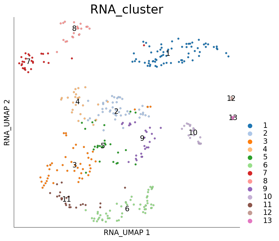
As a result of subsampling the subsampled cells are marked True under the cell metadata column RNA_sketched. We can visualize these cells using plot_layout

[6]:

ds.plot_layout(layout_key='RNA_UMAP', color_by='RNA_cluster', subselection_key='RNA_sketched')

../_images/vignettes_cell_subsampling_tutorial_12_0.png

time: 511 ms (started: 2021-08-22 18:39:51 +00:00)

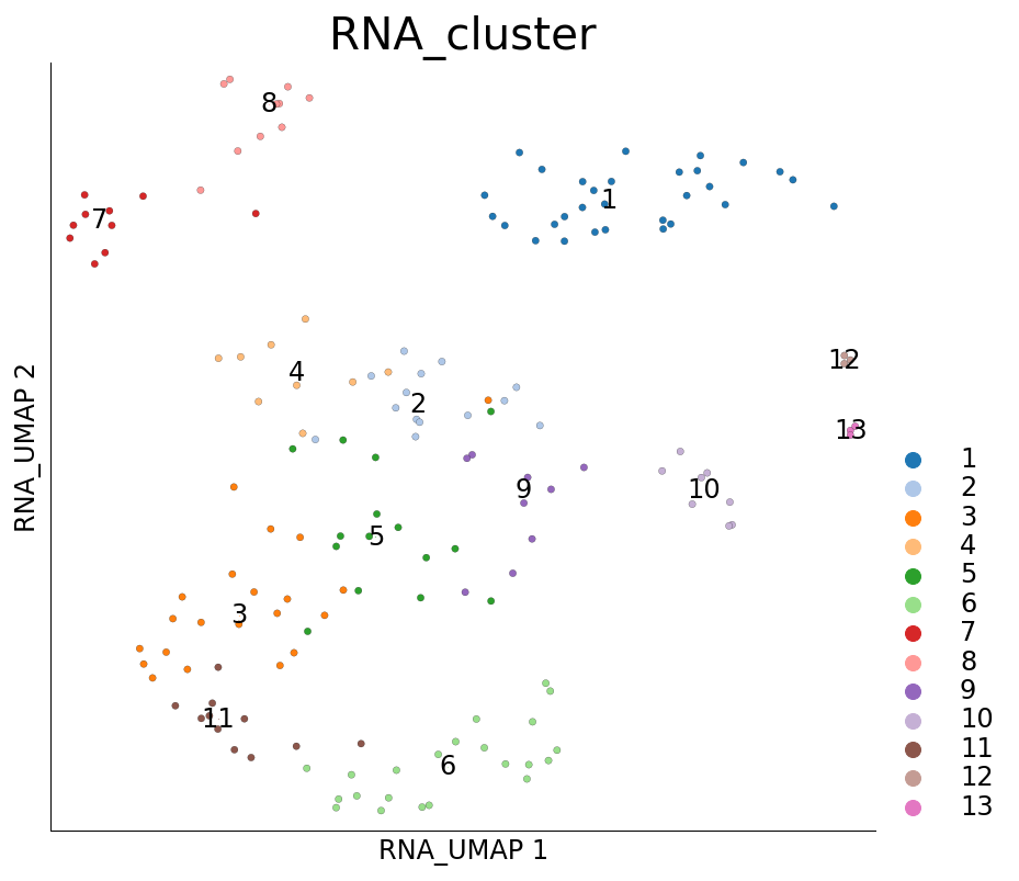
It may also be interesting to visualize the cells that were marked as seed cells used when PCST was run. These cells are marked under the column RNA_sketch_seeds.

[7]:

ds.plot_layout(layout_key='RNA_UMAP', color_by='RNA_cluster', subselection_key='RNA_sketch_seeds')

../_images/vignettes_cell_subsampling_tutorial_14_0.png

time: 412 ms (started: 2021-08-22 18:39:51 +00:00)

4) Intermediate parameters of downsampling¶

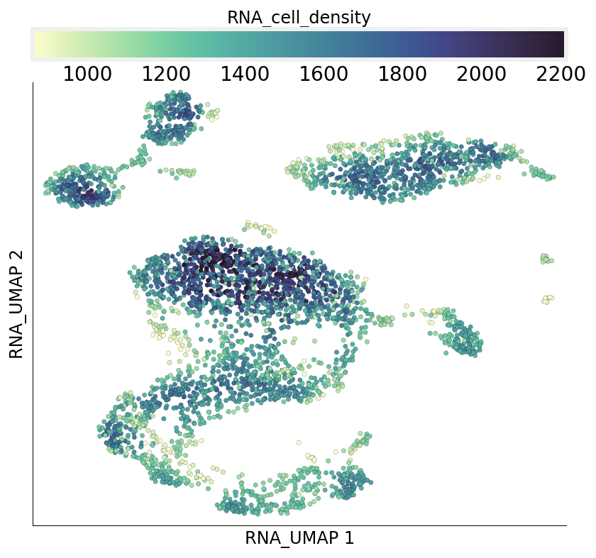
To identify the seed cells, the subsampling algorithm calculates cell densities based on neighbourhood degrees. Regions of higher cell density get a sampling penalty. The neighbourhood degree of individual cells are stored under the column RNA_cell_density.

[8]:

ds.plot_layout(layout_key='RNA_UMAP', color_by='RNA_cell_density')

../_images/vignettes_cell_subsampling_tutorial_17_0.png

time: 696 ms (started: 2021-08-22 18:39:52 +00:00)

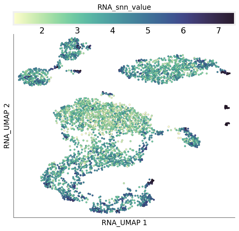
The dowsampling algorithm also identifies regions of the graph where cells form tightly connected groups by calculating mean shared nearest neighbours of each cell’s nieghbours. The tightly connected regions get a sampling award. These values can be accessed from under the cell metadata column RNA_snn_value.

[9]:

ds.plot_layout(layout_key='RNA_UMAP', color_by='RNA_snn_value')

../_images/vignettes_cell_subsampling_tutorial_19_0.png

time: 665 ms (started: 2021-08-22 18:39:52 +00:00)

That is all for this vignette.