Scarf’s basic workflow for scRNA-Seq
This workflow is meant to familiarize users with the Scarf API and how data is internally handled in Scarf. Please checkout the quick start guide if you are interested in the minimal steps required to run the analysis.
[1]:
%load_ext autotime
%config InlineBackend.figure_format = 'retina'

import scarf
scarf.__version__
[1]:
'0.8.5'
time: 952 ms (started: 2021-08-22 18:38:16 +00:00)
Download the count matrix from 10x’s website using the fetch_dataset function. This is a convenience function that stores URLs of datasets that can be downloaded. The save_path parameter allows the data to be saved to a location of choice.
[2]:
scarf.fetch_dataset('tenx_5K_pbmc_rnaseq', save_path='scarf_datasets')
INFO: Download started...
INFO: Download finished! File saved here: /home/docs/checkouts/readthedocs.org/user_builds/scarf/checkouts/0.8.5/docs/source/vignettes/scarf_datasets/tenx_5K_pbmc_rnaseq/data.h5
time: 9.56 s (started: 2021-08-22 18:38:17 +00:00)
2021-08-22 18:38:26 URL:https://storage.googleapis.com/cos-osf-prod-files-de-1/17a47c2d3b323858ae9183e332fa31a01bf130eaa7ca6199ca9d4efe5217374f?response-content-disposition=attachment%3B%20filename%3D%22data.h5%22%3B%20filename%2A%3DUTF-8%27%27data.h5&GoogleAccessId=files-de-1%40cos-osf-prod.iam.gserviceaccount.com&Expires=1629657564&Signature=yQj6UzyzW7fwE8VPQR2cHmtVjC4AztpjrKBxd2h3CDb9J1YxTxCLOj0x%2FMktOiZGF5w3C6e0GjiAjn4GhgpO%2FgUneaRuHITQLAs7RZhlsiyRg6B6jJ1kwALuA3LJ3pe%2FxXBpziNJBW3MiFX0mjM2cSLHjR3AddDBkrqP81TkuU7bfXXNccSNJ7TQL2HtVJ0s8q7tn0CYws9rtiaDyb8jrNsdvc7XmB8clExBVLfyvvMDDLWey35AY%2BRsU5F10%2B%2Fo9sQkLNIPrUSkXDvnP807AAB6F7o4%2FyNNVxQTOl5Gu7e0ZY%2FqyEIKvJyCyink52EaC1sEoXI33VShoDtAsnkHjA%3D%3D [18098007/18098007] -> "/home/docs/checkouts/readthedocs.org/user_builds/scarf/checkouts/0.8.5/docs/source/vignettes/scarf_datasets/tenx_5K_pbmc_rnaseq/data.h5" [1]
1) Format conversion
The first step of the analysis workflow is to convert the file into the Zarr format that is supported by Scarf. We read in the data using CrH5Reader (stands for cellranger H5 reader). The reader object allows quick investigation of the file before the format is converted.
[3]:
reader = scarf.CrH5Reader('scarf_datasets/tenx_5K_pbmc_rnaseq/data.h5', 'rna')
time: 30.1 ms (started: 2021-08-22 18:38:26 +00:00)
We can quickly check the number of cells and features (genes as well as ADT features in this case) present in the file.
[4]:
reader.nCells, reader.nFeatures
[4]:
(5025, 33538)
time: 2.07 ms (started: 2021-08-22 18:38:26 +00:00)
Next we convert the data to the Zarr format that will later on be used by Scarf. For this we use Scarf’s CrToZarr class. This class will first quickly ascertain the type of data to be written and then create a Zarr format file for the data to be written into. CrToZarr takes two mandatory arguments. The first is the cellranger reader, and the other is the name of the output file.
NOTE: When we say zarr file, we actually mean zarr directory because, unlike HDF5, Zarr hierarchy is organized as a directory structure.
[5]:
writer = scarf.CrToZarr(reader, zarr_fn='scarf_datasets/tenx_5K_pbmc_rnaseq/data.zarr',
                        chunk_size=(2000, 1000))
writer.dump(batch_size=1000)
100%|██████████| 6/6 [00:03<00:00, 1.53it/s]
time: 4.04 s (started: 2021-08-22 18:38:26 +00:00)
The next step is to create a Scarf DataStore object. This object will be the primary way to interact with the data and all its constituent assays. When a Zarr file is loaded, Scarf checks if some per-cell statistics have been calculated. If not, then nFeatures (number of features per cell) and nCounts (total sum of feature counts per cell) are calculated. Scarf will also attempt to calculate the percent of mitochondrial and ribosomal content per cell. When we create a DataStore
instance, we can decide to filter out low abundance genes with parameter min_features_per_cell. For example the value of 10 for min_features_per_cell below means that those genes that are present in less than 10 cells will be filtered out.
[6]:
ds = scarf.DataStore('scarf_datasets/tenx_5K_pbmc_rnaseq/data.zarr',
                     nthreads=4, min_features_per_cell=10)
INFO: Setting assay RNA to assay type: RNAassay
INFO: (RNA) Computing nCells and dropOuts
[########################################] | 100% Completed |  0.7s
INFO: (RNA) Computing nCounts
[########################################] | 100% Completed |  0.7s
WARNING: Minimum cell count (502) is lower than size factor multiplier (1000)
INFO: (RNA) Computing nFeatures
[########################################] | 100% Completed |  0.7s
INFO: Computing percentage of RNA_percentMito
[########################################] | 100% Completed |  0.5s
INFO: Computing percentage of RNA_percentRibo
[########################################] | 100% Completed |  0.6s
time: 3.65 s (started: 2021-08-22 18:38:30 +00:00)
2) Cell filtering
We can visualize the per-cell statistics in violin plots before we start filtering cells out.
[7]:
ds.plot_cells_dists()
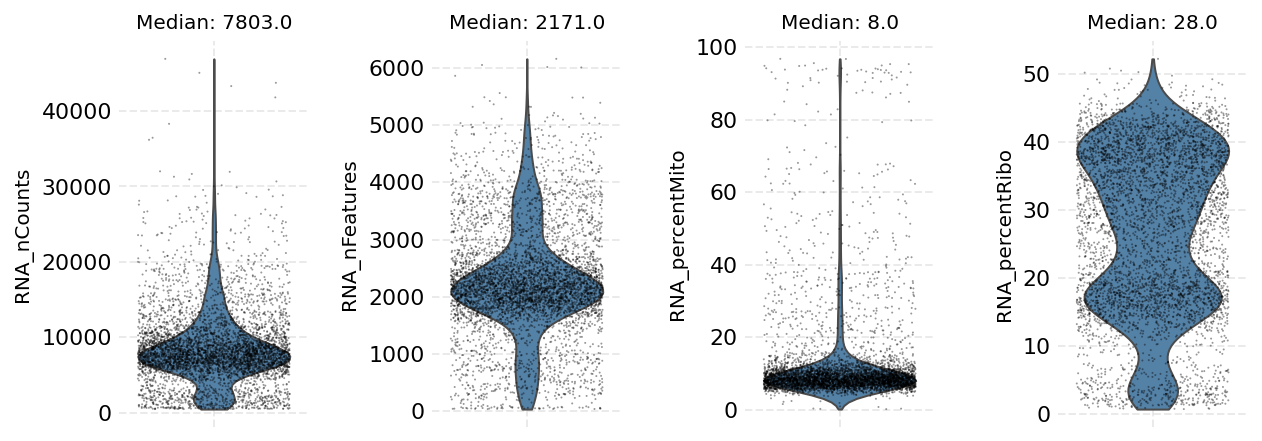
time: 1.24 s (started: 2021-08-22 18:38:34 +00:00)
We can filter cells based on these cell attributes by providing upper and lower threshold values.
[8]:
ds.filter_cells(attrs=['RNA_nCounts', 'RNA_nFeatures', 'RNA_percentMito'],
                highs=[15000, 4000, 15],
                lows=[1000, 500, 0])
INFO: 597 cells flagged for filtering out using attribute RNA_nCounts
INFO: 461 cells flagged for filtering out using attribute RNA_nFeatures
INFO: 612 cells flagged for filtering out using attribute RNA_percentMito
time: 9.92 ms (started: 2021-08-22 18:38:35 +00:00)
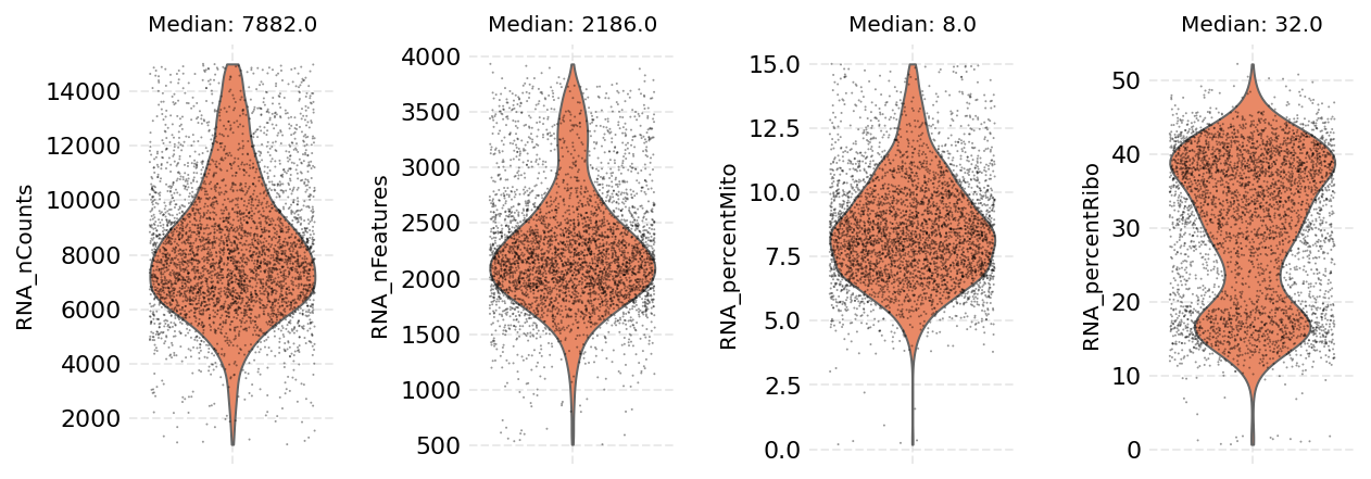
Now we visualize the attributes again after filtering the values.
Note: the ‘I’ value given as the ``cell_key`` attribute signifies the column of the table that is set to ``False`` for cells that were filtered out or ``True`` for cells that are kept.
[9]:
ds.plot_cells_dists(cell_key='I', color='coral')
time: 723 ms (started: 2021-08-22 18:38:35 +00:00)
The data stored under the ‘cellData’ level can easily be accessed using the cells attribute of the DataStore object.
[10]:
ds.cells.head()
[10]:
| I | ids | names | RNA_nCounts | RNA_nFeatures | RNA_percentMito | RNA_percentRibo | |
|---|---|---|---|---|---|---|---|
| 0 | True | AAACCCAAGCGTATGG-1 | AAACCCAAGCGTATGG-1 | 13537.0 | 3503.0 | 10.844353 | 16.783630 |
| 1 | True | AAACCCAGTCCTACAA-1 | AAACCCAGTCCTACAA-1 | 12668.0 | 3381.0 | 5.975687 | 20.034733 |
| 2 | False | AAACCCATCACCTCAC-1 | AAACCCATCACCTCAC-1 | 962.0 | 346.0 | 53.430353 | 2.494802 |
| 3 | True | AAACGCTAGGGCATGT-1 | AAACGCTAGGGCATGT-1 | 5788.0 | 1799.0 | 10.919143 | 28.783690 |
| 4 | True | AAACGCTGTAGGTACG-1 | AAACGCTGTAGGTACG-1 | 13186.0 | 2887.0 | 7.955407 | 35.750038 |
time: 21.7 ms (started: 2021-08-22 18:38:36 +00:00)
NOTE: We strongly discourage directly adding or removing the data from this table as Scarf will not be able to synchronize the changes to the disk. Instead use the methods of the cells attribute. Please refer to the insert, fetch, fetch_all, drop and update_key methods.
3) Feature selection
Similar to the cell table, Scarf also saves the feature level data that can be accessed as below:
[11]:
ds.RNA.feats.head()
[11]:
| I | ids | names | dropOuts | nCells | |
|---|---|---|---|---|---|
| 0 | False | ENSG00000243485 | MIR1302-2HG | 5025 | 0 |
| 1 | False | ENSG00000237613 | FAM138A | 5025 | 0 |
| 2 | False | ENSG00000186092 | OR4F5 | 5025 | 0 |
| 3 | True | ENSG00000238009 | AL627309.1 | 4976 | 49 |
| 4 | False | ENSG00000239945 | AL627309.3 | 5022 | 3 |
time: 18.5 ms (started: 2021-08-22 18:38:36 +00:00)
The feature selection step is performed on the normalized data. The default normalization method for RNAassay-type data is library-size normalization, wherein the count values are divided by the sum of total values for a cell. These values are then multiplied by a scalar factor. The default value of this scalar factor is 1000. However, if the total counts in a cell are less than this value, then on multiplication with this scalar factor the values will be ‘scaled up’ (which is not a desired
behaviour). In the filtering step above, we set the low threshold for RNA_nCounts at 1000, and hence it is safe to use 1000 as a scalar factor. The scalar factor can be set by modifying the sf attribute of the assay. Let’s print the default value of sf
[12]:
ds.RNA.sf
[12]:
1000
time: 1.72 ms (started: 2021-08-22 18:38:36 +00:00)
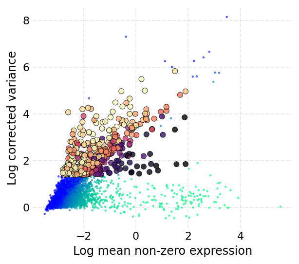
Now the next step is to identify the highly variable genes in the dataset (for the RNA assay). This can be done using the mark_hvgs method of the assay. The parameters govern the min/max variance (corrected) and mean expression threshold for calling genes highly variable.
The variance is corrected by first dividing genes into bins based on their mean expression values. Genes with minimum variance is selected from each bin and a Lowess curve is fitted to the mean-variance trend of these genes. mark_hvgs will by default run on the default assay.
A plot is produced, that for each gene shows the corrected variance on the y-axis and the non-zero mean (means from cells where the gene had a non-zero value) on the x-axis. The genes are colored in two gradients which indicate the number of cells where the gene was expressed. The colors are yellow to dark red for HVGs, and blue to green for non-HVGs.
The mark_hvgs function has a parameter cell_key that dictates which cells to use to identify the HVGs. The default value of this parameter is I, which means it will use all the cells that were not filtered out.
[13]:
ds.mark_hvgs(min_cells=20, top_n=500, min_mean=-3, max_mean=2, max_var=6)
INFO: (RNA) Computing nCells
[########################################] | 100% Completed |  1.1s
INFO: (RNA) Computing normed_tot
[########################################] | 100% Completed |  1.1s
INFO: (RNA) Computing sigmas
[########################################] | 100% Completed |  1.2s
INFO: 497 genes marked as HVGs
time: 5.45 s (started: 2021-08-22 18:38:36 +00:00)
As a result of running mark_hvgs, the feature table now has an extra column I__hvgs which contains a True value for genes marked HVGs. The naming rule in Scarf dictates that cells used to identify HVGs are prepended to the column name (with a double underscore delimiter). Since we did not provide any cell_key parameter the default value was used, i.e. the filtered cells. This resulted in I becoming the prefix.
[14]:
ds.RNA.feats.head()
[14]:
| I | ids | names | I__hvgs | dropOuts | nCells | stats_I_avg | stats_I_c_var__200__0.1 | stats_I_normed_n | stats_I_normed_tot | stats_I_nz_mean | stats_I_sigmas | |
|---|---|---|---|---|---|---|---|---|---|---|---|---|
| 0 | False | ENSG00000243485 | MIR1302-2HG | False | 5025 | 0 | NaN | NaN | NaN | NaN | NaN | NaN |
| 1 | False | ENSG00000237613 | FAM138A | False | 5025 | 0 | NaN | NaN | NaN | NaN | NaN | NaN |
| 2 | False | ENSG00000186092 | OR4F5 | False | 5025 | 0 | NaN | NaN | NaN | NaN | NaN | NaN |
| 3 | True | ENSG00000238009 | AL627309.1 | False | 4976 | 49 | 0.000914 | 1.555434 | 33.0 | 4.593283 | 0.13919 | 0.000196 |
| 4 | False | ENSG00000239945 | AL627309.3 | False | 5022 | 3 | NaN | NaN | NaN | NaN | NaN | NaN |
time: 28.2 ms (started: 2021-08-22 18:38:41 +00:00)
4) Graph creation
Creating a neighbourhood graph of cells is the most critical step in any Scarf workflow. This step internally involves multiple substeps:
data normalization for selected features
linear dimensionality reduction using PCA
creating an approximate nearest neighbour graph index (using the HNSWlib library)
querying cells against this index to identify nearest neighbours for each cell
edge weight computation using the
compute_membership_strengthsfunction from the UMAP packagefitting MiniBatch Kmeans (The kmeans centers are used later, for UMAP initialization)
The make_graph method is responsible for graph construction. Its method takes a mandatory parameter: feat_key. This should be a column in the feature metadata table that indicates which genes to use to create the graph. Since we have already identified the hvgs in the step above, we use those genes. Note that we do not need to write I__hvgs but just hvgs as the value of the parameter. We also supply values for two very important parameters here: k (number of nearest
neighbours to be queried for each cell) and dims (number of PCA dimensions to use for graph construction). n_centroids parameter controls number of clusters to create for the data using the Kmeans algorithm. We perform a more accurate clustering of data in the later steps.
[15]:
ds.make_graph(feat_key='hvgs', k=11, dims=15, n_centroids=100)
INFO: No value provided for parameter `log_transform`. Will use default value: True
INFO: No value provided for parameter `renormalize_subset`. Will use default value: True
INFO: No value provided for parameter `pca_cell_key`. Will use default value: I
INFO: Using PCA for dimension reduction
INFO: No value provided for parameter `ann_metric`. Will use default value: l2
INFO: No value provided for parameter `ann_efc`. Will use default value: min(100, max(k * 3, 50))
INFO: No value provided for parameter `ann_ef`. Will use default value: min(100, max(k * 3, 50))
INFO: No value provided for parameter `ann_m`. Will use default value: 48
INFO: No value provided for parameter `rand_state`. Will use default value: 4466
INFO: No value provided for parameter `local_connectivity`. Will use default value: 1.0
INFO: No value provided for parameter `bandwidth`. Will use default value: 1.5
INFO: Normalizing with feature subset
[########################################] | 100% Completed |  0.6s
Writing data to normed__I__hvgs/data: 100%|██████████| 3/3 [00:00<00:00, 3.58it/s]
INFO: Calculating mean of norm. data
[########################################] | 100% Completed |  0.1s
INFO: Calculating std. dev. of norm. data
[                                        ] | 0% Completed |  0.0s
[########################################] | 100% Completed | 0.1s
Fitting PCA: 100%|██████████| 2/2 [00:00<00:00,  4.02it/s]
Fitting ANN: 100%|██████████| 2/2 [00:00<00:00,  5.49it/s]
Fitting kmeans: 100%|██████████| 2/2 [00:00<00:00,  4.46it/s]
Estimating seed partitions: 100%|██████████| 2/2 [00:00<00:00,  7.98it/s]
INFO: Saving loadings to RNA/normed__I__hvgs/reduction__pca__15__I
INFO: Saving ANN index to RNA/normed__I__hvgs/reduction__pca__15__I/ann__l2__50__50__48__4466
INFO: Saving kmeans clusters to RNA/normed__I__hvgs/reduction__pca__15__I/kmeans__100__4466
Saving KNN graph: 100%|██████████| 2/2 [00:00<00:00, 6.14it/s]
INFO: ANN recall: 99.92%
Smoothening KNN distances: 100%|██████████| 1/1 [00:02<00:00, 2.33s/it]
time: 7.3 s (started: 2021-08-22 18:38:42 +00:00)
5) Low dimensional embedding and clustering
Next we run UMAP on the graph calculated above. Here we will not provide which cell key or feature key to be used, because we want the UMAP to run on all the cells that were not filtered out and with the feature key used to calculate the latest graph. We can provide the parameter values for the UMAP algorithm here.
[16]:
ds.run_umap(fit_n_epochs=250, spread=5, min_dist=1, parallel=True)
/home/docs/checkouts/readthedocs.org/user_builds/scarf/envs/0.8.5/lib/python3.8/site-packages/umap/umap_.py:1330: RuntimeWarning: divide by zero encountered in power
  return 1.0 / (1.0 + a * x ** (2 * b))
        completed  0  /  250 epochs
        completed  25  /  250 epochs
        completed  50  /  250 epochs
        completed  75  /  250 epochs
        completed  100  /  250 epochs
        completed  125  /  250 epochs
        completed  150  /  250 epochs
        completed  175  /  250 epochs
        completed  200  /  250 epochs
        completed  225  /  250 epochs
        completed  0  /  100 epochs
        completed  10  /  100 epochs
        completed  20  /  100 epochs
        completed  30  /  100 epochs
        completed  40  /  100 epochs
        completed  50  /  100 epochs
        completed  60  /  100 epochs
        completed  70  /  100 epochs
        completed  80  /  100 epochs
        completed  90  /  100 epochs
time: 9.73 s (started: 2021-08-22 18:38:49 +00:00)
The UMAP results are saved in the cell metadata table as seen below in columns: RNA_UMAP1 and RNA_UMAP2
[17]:
ds.cells.head()
[17]:
| I | ids | names | RNA_UMAP1 | RNA_UMAP2 | RNA_nCounts | RNA_nFeatures | RNA_percentMito | RNA_percentRibo | |
|---|---|---|---|---|---|---|---|---|---|
| 0 | True | AAACCCAAGCGTATGG-1 | AAACCCAAGCGTATGG-1 | 8.299885 | 17.834124 | 13537.0 | 3503.0 | 10.844353 | 16.783630 |
| 1 | True | AAACCCAGTCCTACAA-1 | AAACCCAGTCCTACAA-1 | 22.908432 | 27.772821 | 12668.0 | 3381.0 | 5.975687 | 20.034733 |
| 2 | False | AAACCCATCACCTCAC-1 | AAACCCATCACCTCAC-1 | NaN | NaN | 962.0 | 346.0 | 53.430353 | 2.494802 |
| 3 | True | AAACGCTAGGGCATGT-1 | AAACGCTAGGGCATGT-1 | -17.693398 | 33.743340 | 5788.0 | 1799.0 | 10.919143 | 28.783690 |
| 4 | True | AAACGCTGTAGGTACG-1 | AAACGCTGTAGGTACG-1 | -9.829469 | 10.378865 | 13186.0 | 2887.0 | 7.955407 | 35.750038 |
time: 21.3 ms (started: 2021-08-22 18:38:59 +00:00)
plot_layout is a versatile method to create a scatter plot using Scarf. Here we can plot the UMAP coordinates of all the non-filtered out cells.
[18]:
ds.plot_layout(layout_key='RNA_UMAP')
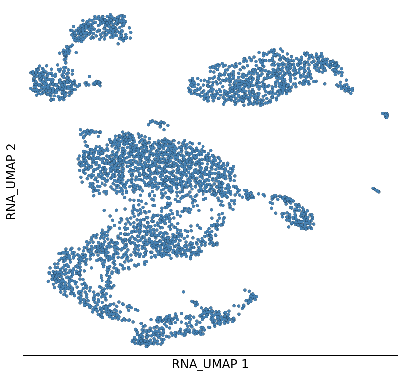
time: 234 ms (started: 2021-08-22 18:38:59 +00:00)
plot_layout can be used to easily visualize data from any column of the cell metadata table. Next, we visualize the number of genes expressed in each cell.
[19]:
ds.plot_layout(layout_key='RNA_UMAP', color_by='RNA_nCounts', cmap='coolwarm')
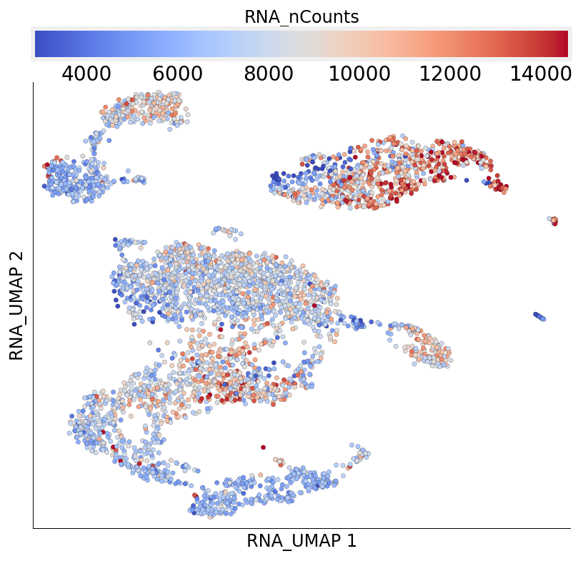
time: 681 ms (started: 2021-08-22 18:38:59 +00:00)
There has been a lot of discussion over the choice of non-linear dimensionality reduction for single-cell data. tSNE was initially considered an excellent solution, but has gradually lost out to UMAP because the magnitude of relations between the clusters cannot easily be discerned in a tSNE plot. Scarf contains an implementation of tSNE that runs directly on the graph structure of cells. So, essentially the same data that was used to create the UMAP and clustering is used.
[20]:
ds.run_tsne(alpha=10, box_h=1, early_iter=250, max_iter=500, parallel=True)
Saving KNN matrix in MTX format: 100%|██████████| 4/4 [00:00<00:00, 38.48it/s]
ERROR: SG-tSNE failed, possibly due to missing libraries or file permissions. SG-tSNE currently fails on readthedocs
time: 152 ms (started: 2021-08-22 18:39:00 +00:00)
sgtsne: error while loading shared libraries: libmetis.so.5: cannot open shared object file: No such file or directory
NOTE: The tSNE implementation is currently not supported on Windows.
[21]:
# Here we run plot_layout under exception catching because if you are not on Linux then the `run_tnse` would have failed.
try:
    ds.plot_layout(layout_key='RNA_tSNE')
except KeyError:
    print ("'RNA_tSNE1' not found in MetaData")
'RNA_tSNE1' not found in MetaData
time: 2.63 ms (started: 2021-08-22 18:39:00 +00:00)
6) Cell clustering
Identifying clusters of cells is one of the central tenets of single cell approaches. Scarf includes two graph clustering methods and any (or even both) can be used on the dataset. The methods start with the same graph as the UMAP algorithm above to minimize the disparity between the UMAP and clustering results. The two clustering methods are:
Paris: This is the default clustering algorithm.
Leiden: Leiden is a widely used graph clustering algorithm in single-cell genomics.
Paris is the default algorithm in Scarf due to its ability to highlight cluster relationships. Paris is a hierarchical graph clustering algorithm that is based on node pair sampling. Paris creates a dendrogram of cells which can then be cut to obtain desired number of clusters. The advantage of using Paris, especially in the larger datasets, is that once the dendrogram has been created one can change the desired number of clusters with minimal computation overhead.
[22]:
# We start with Leiden clustering
ds.run_leiden_clustering(resolution=0.5)
time: 96.6 ms (started: 2021-08-22 18:39:00 +00:00)
We can visualize the results using the plot_layout method again. Here we plot both UMAP and colour cells based on their cluster identity, as obtained using Leiden clustering.
[23]:
ds.plot_layout(layout_key='RNA_UMAP', color_by='RNA_leiden_cluster')
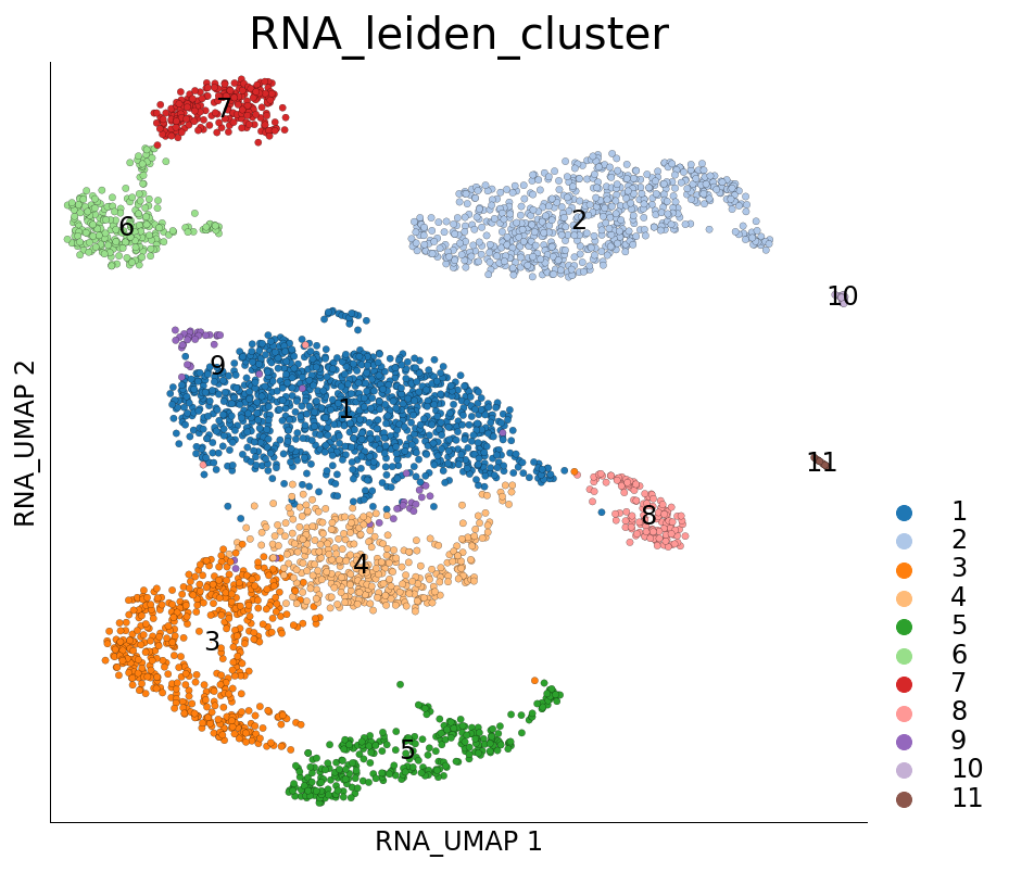
time: 493 ms (started: 2021-08-22 18:39:00 +00:00)
The results of the clustering algorithm are saved in the cell metadata table. In this case, they have been saved under the column name RNA_leiden_cluster.
[24]:
ds.cells.head()
[24]:
| I | ids | names | RNA_UMAP1 | RNA_UMAP2 | RNA_leiden_cluster | RNA_nCounts | RNA_nFeatures | RNA_percentMito | RNA_percentRibo | |
|---|---|---|---|---|---|---|---|---|---|---|
| 0 | True | AAACCCAAGCGTATGG-1 | AAACCCAAGCGTATGG-1 | 8.299885 | 17.834124 | 2 | 13537.0 | 3503.0 | 10.844353 | 16.783630 |
| 1 | True | AAACCCAGTCCTACAA-1 | AAACCCAGTCCTACAA-1 | 22.908432 | 27.772821 | 2 | 12668.0 | 3381.0 | 5.975687 | 20.034733 |
| 2 | False | AAACCCATCACCTCAC-1 | AAACCCATCACCTCAC-1 | NaN | NaN | -1 | 962.0 | 346.0 | 53.430353 | 2.494802 |
| 3 | True | AAACGCTAGGGCATGT-1 | AAACGCTAGGGCATGT-1 | -17.693398 | 33.743340 | 7 | 5788.0 | 1799.0 | 10.919143 | 28.783690 |
| 4 | True | AAACGCTGTAGGTACG-1 | AAACGCTGTAGGTACG-1 | -9.829469 | 10.378865 | 1 | 13186.0 | 2887.0 | 7.955407 | 35.750038 |
time: 25.4 ms (started: 2021-08-22 18:39:00 +00:00)
We can export the Leiden cluster information into a pandas dataframe. Setting key to I makes sure that we do not include the data for cells that were filtered out.
[25]:
leiden_clusters = ds.cells.to_pandas_dataframe(['RNA_leiden_cluster'], key='I')
leiden_clusters.head()
[25]:
| RNA_leiden_cluster | |
|---|---|
| 0 | 2 |
| 1 | 2 |
| 3 | 7 |
| 4 | 1 |
| 6 | 5 |
time: 7.87 ms (started: 2021-08-22 18:39:00 +00:00)
Now we run Paris clustering algorithm using run_clustering method. Paris clustering requires only one parameter: n_clusters, which determines the number of clusters to create. Here we set the number of clusters same as that were obtained using Leiden clustering.leiden_clusters.nunique()
[26]:
ds.run_clustering(n_clusters=leiden_clusters.nunique()[0])
time: 282 ms (started: 2021-08-22 18:39:00 +00:00)
Visualizing Paris clusters
[27]:
ds.plot_layout(layout_key='RNA_UMAP', color_by='RNA_cluster')
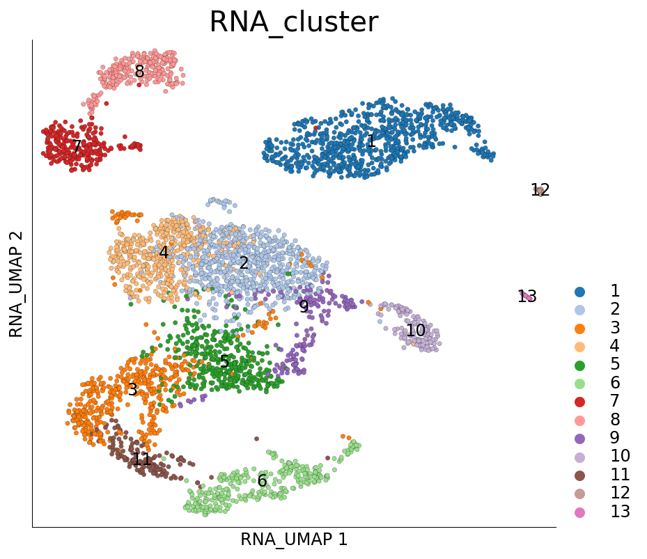
time: 515 ms (started: 2021-08-22 18:39:01 +00:00)
Discerning similarity between clusters can be difficult from visual inspection alone, especially for tSNE plots. plot_cluster_tree function plots the relationship between clusters as a binary tree. This tree is simply a condensation of the dendrogram obtained using Paris clustering.
[28]:
ds.plot_cluster_tree(cluster_key='RNA_cluster', width=1)
Constructing graph from dendrogram: 100%|██████████| 3939/3939 [00:00<00:00, 53793.96it/s]
Identifying the top node for cluster: 100%|██████████| 13/13 [00:00<00:00, 569.49it/s]
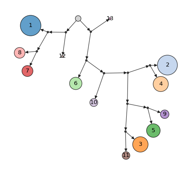
time: 627 ms (started: 2021-08-22 18:39:01 +00:00)
The tree is free form (i.e the position of clusters doesn’t convey any meaning) but allows inspection of cluster similarity based on branching pattern. The sizes of clusters indicate the number of cells present in each cluster. The tree starts from the root node (black dot with no incoming edges).
7) Marker gene identification
Now we can identify the genes that are differentially expressed between the clusters using the run_marker_search method. The method to identify the differentially expressed genes in Scarf is optimized to obtain quick results. We have not compared the sensitivity of our method to other differential expression-detecting methods. We expect specialized methods to be more sensitive and accurate to varying degrees. Our method is designed to quickly obtain key marker genes for populations from a
large dataset. For each gene individually, following steps are carried out:
Expression values are converted to ranks (dense format) across cells.
A mean of ranks is calculated for each group of cells.
The mean value for each group is divided by the sum of mean values to obtain the ‘specificity score’.
The gene is saved as a marker gene if it’s specificity score is higher than a given threshold.
This method does not perform any statistical test of significance and uses ‘specificity score’ as a measure of importance of each gene for a cluster.
[29]:
ds.run_marker_search(group_key='RNA_cluster', threshold=0.25)
Finding markers: 100%|██████████| 272/272 [00:16<00:00, 16.72it/s]
time: 16.4 s (started: 2021-08-22 18:39:02 +00:00)
Using the plot_marker_heatmap method, we can also plot a heatmap with the top marker genes from each cluster. The method will calculate the mean expression value for each gene from each cluster.
[30]:
ds.plot_marker_heatmap(group_key='RNA_cluster', topn=5, figsize=(5, 9))
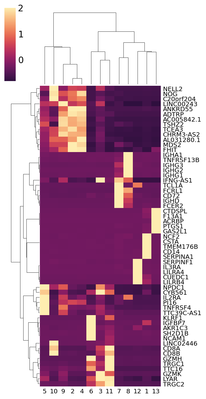
time: 1.94 s (started: 2021-08-22 18:39:18 +00:00)
The markers list for specific clusters can be obtained like this:
[31]:
ds.get_markers(group_key='RNA_cluster', group_id='1')
[31]:
| score | names | |
|---|---|---|
| ids | ||
| ENSG00000121552 | 0.949142 | CSTA |
| ENSG00000170458 | 0.947154 | CD14 |
| ENSG00000106565 | 0.945043 | TMEM176B |
| ENSG00000197249 | 0.945023 | SERPINA1 |
| ENSG00000116701 | 0.943234 | NCF2 |
| ... | ... | ... |
| ENSG00000144802 | 0.251001 | NFKBIZ |
| ENSG00000163661 | 0.250964 | PTX3 |
| ENSG00000100605 | 0.250697 | ITPK1 |
| ENSG00000182095 | 0.250591 | TNRC18 |
| ENSG00000163131 | 0.250493 | CTSS |
655 rows × 2 columns
time: 64.3 ms (started: 2021-08-22 18:39:20 +00:00)
We can directly visualize the expression values for a gene of interest. It is usually a good idea to visually confirm the gene expression pattern across the cells at least this way.
[32]:
ds.plot_layout(layout_key='RNA_UMAP', color_by='CD14')
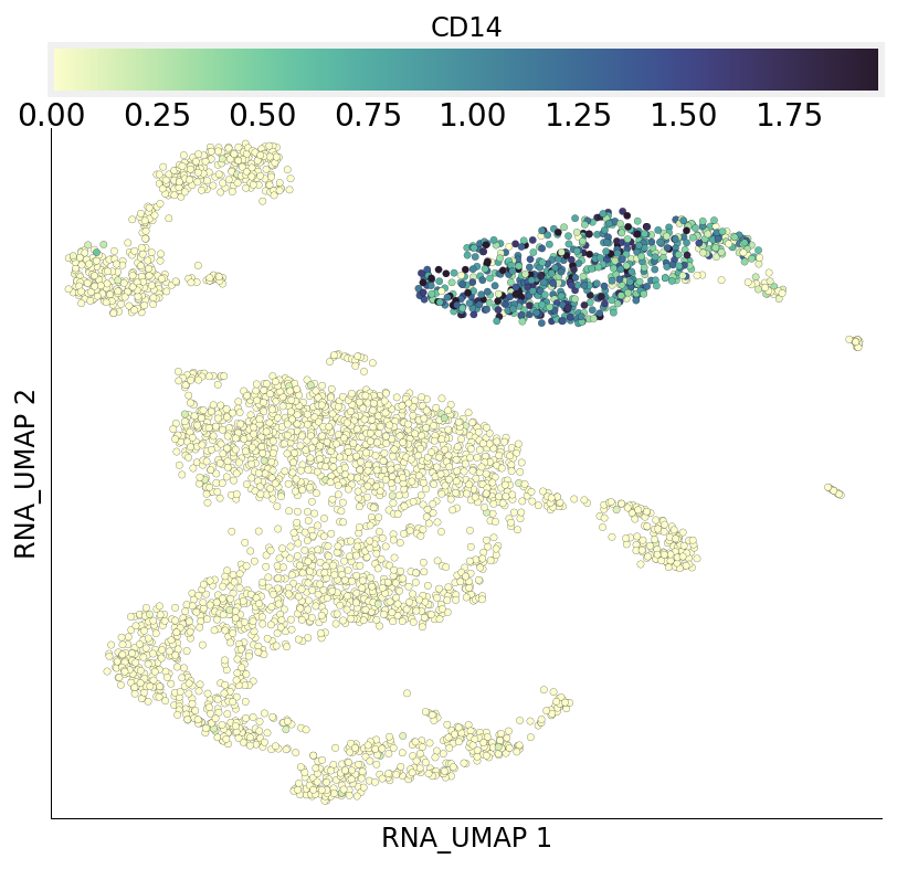
time: 852 ms (started: 2021-08-22 18:39:20 +00:00)
That is all for this vignette.