Handling datasets with multiple modalities#
%load_ext autotime

import scarf
scarf.__version__
'0.23.5'
time: 1.67 s (started: 2023-05-24 14:47:57 +00:00)
1) Fetch and convert data#
For this tutorial we will use CITE-Seq data from 10x genomics. This dataset contains two modalities: gene expression and surface protein abundance. Throughout this tutorial we will refer to gene expression modality as RNA and surface protein as ADT. We start by downloading the data and converting it into Zarr format:
scarf.fetch_dataset(
    'tenx_8K_pbmc_citeseq',
    save_path='scarf_datasets'
)
time: 15.8 s (started: 2023-05-24 14:47:59 +00:00)
reader = scarf.CrH5Reader(
    'scarf_datasets/tenx_8K_pbmc_citeseq/data.h5'
)
time: 55.9 ms (started: 2023-05-24 14:48:14 +00:00)
We can also quickly check the different kinds of assays present in the file and the number of features from each of them.
reader.assayFeats
| RNA | ADT | |
|---|---|---|
| type | Gene Expression | Antibody Capture |
| start | 0 | 33538 |
| end | 33538 | 33555 |
| nFeatures | 33538 | 17 |
time: 11.8 ms (started: 2023-05-24 14:48:15 +00:00)
The nFeatures column shows the number of features present in each assay. CrH5Reader will automatically pull this information from H5 file and rename the ‘Gene Expression’ assay to RNA. Here it also found another assay: ‘Antibody Capture’ and named it to assay2. We will rename this to ADT.
reader.rename_assays({'assay2': 'ADT'})
reader.assayFeats
| RNA | ADT | |
|---|---|---|
| type | Gene Expression | Antibody Capture |
| start | 0 | 33538 |
| end | 33538 | 33555 |
| nFeatures | 33538 | 17 |
time: 8.95 ms (started: 2023-05-24 14:48:15 +00:00)
Now the data is converted into Zarr format. Like single assay datasets, all the data is saved under one Zarr file.
writer = scarf.CrToZarr(
    reader,
    zarr_fn='scarf_datasets/tenx_8K_pbmc_citeseq/data.zarr',
    chunk_size=(2000, 1000),
)
writer.dump(batch_size=1000)
time: 8.82 s (started: 2023-05-24 14:48:15 +00:00)
2) Create a multimodal DataStore#
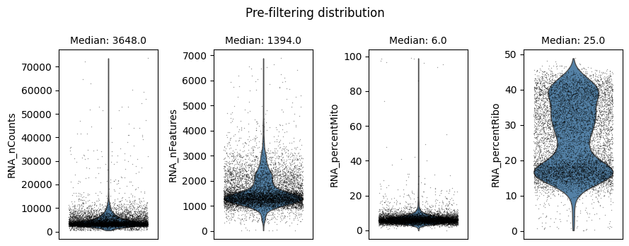
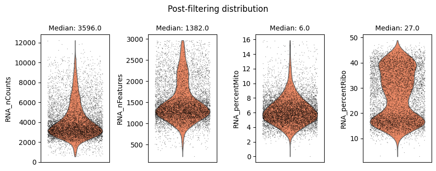
The next step is to create a Scarf DataStore object. This object will be the primary way to interact with the data and all its constituent assays. The first time a Zarr file is loaded, we need to set the default assay. Here we set the ‘RNA’ assay as the default assay. When a Zarr file is loaded, Scarf checks if some per-cell statistics have been calculated. If not, then nFeatures (number of features per cell) and nCounts (total sum of feature counts per cell) are calculated. Scarf will also attempt to calculate the percent of mitochondrial and ribosomal content per cell.
ds = scarf.DataStore(
    'scarf_datasets/tenx_8K_pbmc_citeseq/data.zarr',
    default_assay='RNA',
    nthreads=4
)
WARNING: Minimum cell count (501) is lower than size factor multiplier (1000)
time: 8.68 s (started: 2023-05-24 14:48:23 +00:00)
We can print out the DataStore object to get an overview of all the assays stored.
ds
DataStore has 7865 (7865) cells with 2 assays: ADT RNA
   Cell metadata:
            'I', 'ids', 'names', 'ADT_nCounts', 'ADT_nFeatures',
            'RNA_nCounts', 'RNA_nFeatures', 'RNA_percentMito', 'RNA_percentRibo'
   ADT assay has 17 (17) features and following metadata:
            'I', 'ids', 'names', 'dropOuts', 'nCells',

   RNA assay has 13832 (33538) features and following metadata:
            'I', 'ids', 'names', 'dropOuts', 'nCells',
time: 16.3 ms (started: 2023-05-24 14:48:32 +00:00)
Feature attribute tables for each of the assays can be accessed like this:
ds.RNA.feats.head()
| I | ids | names | dropOuts | nCells | |
|---|---|---|---|---|---|
| 0 | False | ENSG00000243485 | MIR1302-2HG | 7865 | 0 |
| 1 | False | ENSG00000237613 | FAM138A | 7865 | 0 |
| 2 | False | ENSG00000186092 | OR4F5 | 7865 | 0 |
| 3 | False | ENSG00000238009 | AL627309.1 | 7853 | 12 |
| 4 | False | ENSG00000239945 | AL627309.3 | 7865 | 0 |
time: 31.4 ms (started: 2023-05-24 14:48:32 +00:00)
ds.ADT.feats.head()
| I | ids | names | dropOuts | nCells | |
|---|---|---|---|---|---|
| 0 | True | CD3 | CD3_TotalSeqB | 1 | 7864 |
| 1 | True | CD4 | CD4_TotalSeqB | 1 | 7864 |
| 2 | True | CD8a | CD8a_TotalSeqB | 2 | 7863 |
| 3 | True | CD14 | CD14_TotalSeqB | 1 | 7864 |
| 4 | True | CD15 | CD15_TotalSeqB | 1 | 7864 |
time: 26.6 ms (started: 2023-05-24 14:48:32 +00:00)
Cell filtering is performed based on the default assay. Here we use the auto_filter_cells method of the DataStore to filter low quality cells.
ds.auto_filter_cells()
INFO: 154 cells flagged for filtering out using attribute RNA_nCounts
INFO: 326 cells flagged for filtering out using attribute RNA_nFeatures
INFO: 119 cells flagged for filtering out using attribute RNA_percentMito
INFO: 21 cells flagged for filtering out using attribute RNA_percentRibo
time: 5.01 s (started: 2023-05-24 14:48:32 +00:00)
3) Process gene expression modality#
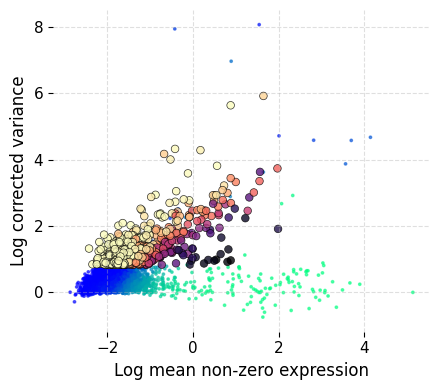
Now we process the RNA assay to perform feature selection, create KNN graph, run UMAP reduction and clustering. These steps are same as shown in the basic workflow for scRNA-Seq data.
ds.mark_hvgs(
    min_cells=20,
    top_n=1000,
    min_mean=-3,
    max_mean=2,
    max_var=6
)

ds.make_graph(
    feat_key='hvgs',
    k=21,
    dims=15,
    n_centroids=100
)

ds.run_umap(
    n_epochs=250,
    spread=5,
    min_dist=1,
    parallel=True
)

ds.run_leiden_clustering(resolution=1)
INFO: 997 genes marked as HVGs
/home/docs/checkouts/readthedocs.org/user_builds/scarf/envs/0.23.5/lib/python3.8/site-packages/sklearn/cluster/_kmeans.py:870: FutureWarning: The default value of `n_init` will change from 3 to 'auto' in 1.4. Set the value of `n_init` explicitly to suppress the warning
  warnings.warn(
/home/docs/checkouts/readthedocs.org/user_builds/scarf/envs/0.23.5/lib/python3.8/site-packages/umap/distances.py:1063: NumbaDeprecationWarning: The 'nopython' keyword argument was not supplied to the 'numba.jit' decorator. The implicit default value for this argument is currently False, but it will be changed to True in Numba 0.59.0. See https://numba.readthedocs.io/en/stable/reference/deprecation.html#deprecation-of-object-mode-fall-back-behaviour-when-using-jit for details.
  @numba.jit()
/home/docs/checkouts/readthedocs.org/user_builds/scarf/envs/0.23.5/lib/python3.8/site-packages/umap/distances.py:1071: NumbaDeprecationWarning: The 'nopython' keyword argument was not supplied to the 'numba.jit' decorator. The implicit default value for this argument is currently False, but it will be changed to True in Numba 0.59.0. See https://numba.readthedocs.io/en/stable/reference/deprecation.html#deprecation-of-object-mode-fall-back-behaviour-when-using-jit for details.
  @numba.jit()
/home/docs/checkouts/readthedocs.org/user_builds/scarf/envs/0.23.5/lib/python3.8/site-packages/umap/distances.py:1086: NumbaDeprecationWarning: The 'nopython' keyword argument was not supplied to the 'numba.jit' decorator. The implicit default value for this argument is currently False, but it will be changed to True in Numba 0.59.0. See https://numba.readthedocs.io/en/stable/reference/deprecation.html#deprecation-of-object-mode-fall-back-behaviour-when-using-jit for details.
  @numba.jit()
/home/docs/checkouts/readthedocs.org/user_builds/scarf/envs/0.23.5/lib/python3.8/site-packages/umap/umap_.py:660: NumbaDeprecationWarning: The 'nopython' keyword argument was not supplied to the 'numba.jit' decorator. The implicit default value for this argument is currently False, but it will be changed to True in Numba 0.59.0. See https://numba.readthedocs.io/en/stable/reference/deprecation.html#deprecation-of-object-mode-fall-back-behaviour-when-using-jit for details.
  @numba.jit()
INFO: ANN recall: 96.19%
time: 1min 19s (started: 2023-05-24 14:48:37 +00:00)
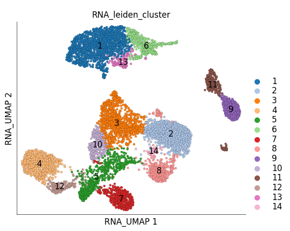
ds.plot_layout(
    layout_key='RNA_UMAP',
    color_by='RNA_leiden_cluster',
    cmap='tab20'
)
time: 1.03 s (started: 2023-05-24 14:49:56 +00:00)
4) Process protein surface abundance modality#
We will now perform similar steps as RNA for the ADT data. Since ADT panels are often custom designed, we will not perform any feature selection step. This particular data contains some control antibodies which we should filter out before downstream analysis.
ds.ADT.feats.head(n=ds.ADT.feats.N)
| I | ids | names | dropOuts | nCells | |
|---|---|---|---|---|---|
| 0 | True | CD3 | CD3_TotalSeqB | 1 | 7864 |
| 1 | True | CD4 | CD4_TotalSeqB | 1 | 7864 |
| 2 | True | CD8a | CD8a_TotalSeqB | 2 | 7863 |
| 3 | True | CD14 | CD14_TotalSeqB | 1 | 7864 |
| 4 | True | CD15 | CD15_TotalSeqB | 1 | 7864 |
| 5 | True | CD16 | CD16_TotalSeqB | 1 | 7864 |
| 6 | True | CD56 | CD56_TotalSeqB | 1 | 7864 |
| 7 | True | CD19 | CD19_TotalSeqB | 163 | 7702 |
| 8 | True | CD25 | CD25_TotalSeqB | 4 | 7861 |
| 9 | True | CD45RA | CD45RA_TotalSeqB | 1 | 7864 |
| 10 | True | CD45RO | CD45RO_TotalSeqB | 1 | 7864 |
| 11 | True | PD-1 | PD-1_TotalSeqB | 2 | 7863 |
| 12 | True | TIGIT | TIGIT_TotalSeqB | 16 | 7849 |
| 13 | True | CD127 | CD127_TotalSeqB | 3 | 7862 |
| 14 | True | IgG2a | IgG2a_control_TotalSeqB | 26 | 7839 |
| 15 | True | IgG1 | IgG1_control_TotalSeqB | 9 | 7856 |
| 16 | True | IgG2b | IgG2b_control_TotalSeqB | 226 | 7639 |
time: 33.9 ms (started: 2023-05-24 14:49:57 +00:00)
We can manually filter out the control antibodies by updating I to be False for those features. To do so we first extract the names of all the ADT features like below:
adt_names = ds.ADT.feats.to_pandas_dataframe(['names'])['names']
adt_names
0               CD3_TotalSeqB
1               CD4_TotalSeqB
2              CD8a_TotalSeqB
3              CD14_TotalSeqB
4              CD15_TotalSeqB
5              CD16_TotalSeqB
6              CD56_TotalSeqB
7              CD19_TotalSeqB
8              CD25_TotalSeqB
9            CD45RA_TotalSeqB
10           CD45RO_TotalSeqB
11             PD-1_TotalSeqB
12            TIGIT_TotalSeqB
13            CD127_TotalSeqB
14    IgG2a_control_TotalSeqB
15     IgG1_control_TotalSeqB
16    IgG2b_control_TotalSeqB
Name: names, dtype: object
time: 17.1 ms (started: 2023-05-24 14:49:57 +00:00)
The ADT features with ‘control’ in name are designated as control antibodies. You can have your own selection criteria here. The aim here is to create a boolean array that has True value for features to be removed.
is_control = adt_names.str.contains('control').values
is_control
array([False, False, False, False, False, False, False, False, False,
       False, False, False, False, False,  True,  True,  True])
time: 5.37 ms (started: 2023-05-24 14:49:57 +00:00)
Now we update I to remove the control features. update_key method takes a boolean array and disables the features that have False value. So we invert the above created array (using ~) before providing it to update_key. The second parameter for update_key denotes which feature table boolean column to modify, I in this case.
ds.ADT.feats.update_key(~is_control, 'I')
ds.ADT.feats.head(n=ds.ADT.feats.N)
| I | ids | names | dropOuts | nCells | |
|---|---|---|---|---|---|
| 0 | True | CD3 | CD3_TotalSeqB | 1 | 7864 |
| 1 | True | CD4 | CD4_TotalSeqB | 1 | 7864 |
| 2 | True | CD8a | CD8a_TotalSeqB | 2 | 7863 |
| 3 | True | CD14 | CD14_TotalSeqB | 1 | 7864 |
| 4 | True | CD15 | CD15_TotalSeqB | 1 | 7864 |
| 5 | True | CD16 | CD16_TotalSeqB | 1 | 7864 |
| 6 | True | CD56 | CD56_TotalSeqB | 1 | 7864 |
| 7 | True | CD19 | CD19_TotalSeqB | 163 | 7702 |
| 8 | True | CD25 | CD25_TotalSeqB | 4 | 7861 |
| 9 | True | CD45RA | CD45RA_TotalSeqB | 1 | 7864 |
| 10 | True | CD45RO | CD45RO_TotalSeqB | 1 | 7864 |
| 11 | True | PD-1 | PD-1_TotalSeqB | 2 | 7863 |
| 12 | True | TIGIT | TIGIT_TotalSeqB | 16 | 7849 |
| 13 | True | CD127 | CD127_TotalSeqB | 3 | 7862 |
| 14 | False | IgG2a | IgG2a_control_TotalSeqB | 26 | 7839 |
| 15 | False | IgG1 | IgG1_control_TotalSeqB | 9 | 7856 |
| 16 | False | IgG2b | IgG2b_control_TotalSeqB | 226 | 7639 |
time: 33.9 ms (started: 2023-05-24 14:49:57 +00:00)
Assays named ADT are automatically created as objects of the ADTassay class, which uses CLR (centred log ratio) normalization as the default normalization method.
print (ds.ADT)
print (ds.ADT.normMethod.__name__)
ADTassay ADT with 14(17) features
norm_clr
time: 2.21 ms (started: 2023-05-24 14:49:58 +00:00)
Now we are ready to create a KNN graph of cells using only ADT data. Here we will use all the features (except those that were filtered out) and that is why we use I as value for feat_key. It is important to note the value for from_assay parameter which has now been set to ADT. If no value is provided for from_assay then it is automatically set to the default assay. By setting dims to 0 we disable dimension reduction.
ds.make_graph(
    from_assay='ADT',
    feat_key='I',
    k=21,
    dims=0,
    n_centroids=100
)
/home/docs/checkouts/readthedocs.org/user_builds/scarf/envs/0.23.5/lib/python3.8/site-packages/sklearn/cluster/_kmeans.py:870: FutureWarning: The default value of `n_init` will change from 3 to 'auto' in 1.4. Set the value of `n_init` explicitly to suppress the warning
  warnings.warn(
INFO: ANN recall: 99.99%
time: 3.42 s (started: 2023-05-24 14:49:58 +00:00)
UMAP and clustering can be run on ADT assay by simply setting from_assay parameter value to ‘ADT’:
ds.run_umap(
    from_assay='ADT',
    n_epochs=250,
    spread=5,
    min_dist=1,
    parallel=True
)

ds.run_leiden_clustering(
    from_assay='ADT',
    resolution=1
)
time: 32.2 s (started: 2023-05-24 14:50:01 +00:00)
If we now check the cell attribute table, we will find the UMAP coordinates and clusters calculated using ADT assay:
ds.cells.head()
| I | ids | names | ADT_UMAP1 | ADT_UMAP2 | ADT_leiden_cluster | ADT_nCounts | ADT_nFeatures | RNA_UMAP1 | RNA_UMAP2 | RNA_leiden_cluster | RNA_nCounts | RNA_nFeatures | RNA_percentMito | RNA_percentRibo | |
|---|---|---|---|---|---|---|---|---|---|---|---|---|---|---|---|
| 0 | True | AAACCCAAGATTGTGA-1 | AAACCCAAGATTGTGA-1 | -22.042093 | 15.468054 | 5 | 981.0 | 17.0 | -19.306347 | 25.692945 | 1 | 6160.0 | 2194.0 | 8.668831 | 15.259740 |
| 1 | True | AAACCCACATCGGTTA-1 | AAACCCACATCGGTTA-1 | -8.776048 | 20.052792 | 14 | 1475.0 | 17.0 | -18.741245 | 23.497496 | 1 | 6713.0 | 2093.0 | 6.316103 | 19.037688 |
| 2 | True | AAACCCAGTACCGCGT-1 | AAACCCAGTACCGCGT-1 | -13.516581 | 21.566793 | 5 | 7149.0 | 17.0 | -6.967236 | 23.046961 | 1 | 3637.0 | 1518.0 | 8.056090 | 16.002200 |
| 3 | True | AAACCCAGTATCGAAA-1 | AAACCCAGTATCGAAA-1 | 25.298540 | 19.771112 | 3 | 6831.0 | 17.0 | -31.555559 | -11.693686 | 4 | 1244.0 | 737.0 | 9.003215 | 18.729904 |
| 4 | True | AAACCCAGTCGTCATA-1 | AAACCCAGTCGTCATA-1 | 25.568506 | 17.301783 | 3 | 6839.0 | 17.0 | -33.793198 | -16.785084 | 4 | 2611.0 | 1240.0 | 6.204519 | 16.353887 |
time: 60.2 ms (started: 2023-05-24 14:50:33 +00:00)
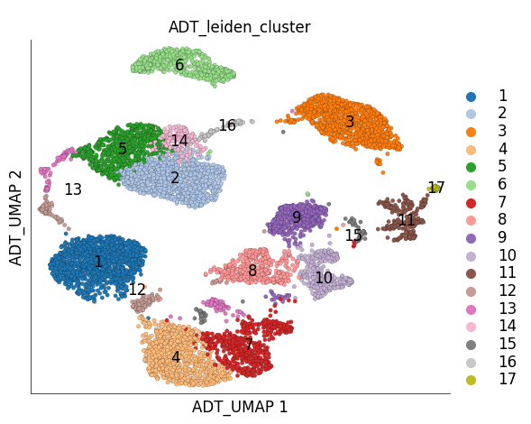
Visualizing the UMAP and clustering calcualted using ADT only:
ds.plot_layout(
    layout_key='ADT_UMAP',
    color_by='ADT_leiden_cluster',
    cmap='tab20'
)
time: 1.12 s (started: 2023-05-24 14:50:33 +00:00)
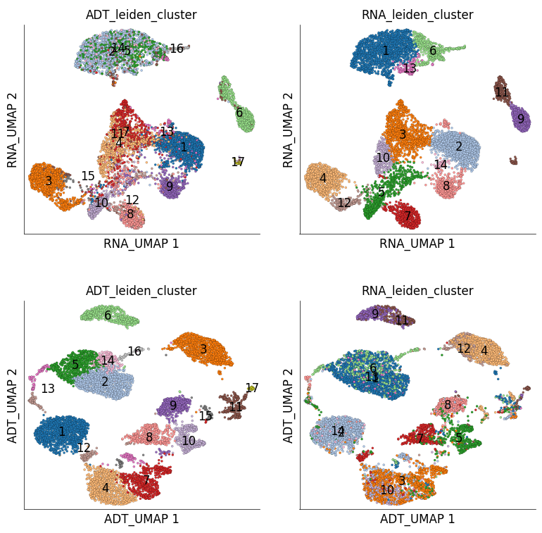
5) Cross modality comparison#
It is generally of interest to see how different modalities corroborate each other.
# UMAP on RNA and coloured with clusters calculated on ADT
ds.plot_layout(
    layout_key=['RNA_UMAP', 'ADT_UMAP'],
    color_by=['ADT_leiden_cluster', 'RNA_leiden_cluster'],
    cmap='tab20',
    width=4,
    height=4,
    n_columns=2,
    point_size=5,
    legend_onside=False
)
time: 2.07 s (started: 2023-05-24 14:50:34 +00:00)
We can quantify the overlap of cells between RNA and ADT clusters. The following table has ADT clusters on columns and RNA clusters on rows. This table shows a cross tabulation of cells across the clustering from the two modalities.
import pandas as pd

df = pd.crosstab(
    ds.cells.fetch('RNA_leiden_cluster'),
    ds.cells.fetch('ADT_leiden_cluster')
)
df
| col_0 | 1 | 2 | 3 | 4 | 5 | 6 | 7 | 8 | 9 | 10 | 11 | 12 | 13 | 14 | 15 | 16 | 17 |
|---|---|---|---|---|---|---|---|---|---|---|---|---|---|---|---|---|---|
| row_0 | |||||||||||||||||
| 1 | 0 | 756 | 13 | 4 | 362 | 2 | 5 | 13 | 0 | 3 | 62 | 0 | 1 | 113 | 15 | 0 | 0 |
| 2 | 967 | 0 | 0 | 50 | 0 | 1 | 27 | 0 | 26 | 1 | 13 | 11 | 49 | 0 | 0 | 0 | 0 |
| 3 | 20 | 0 | 0 | 423 | 0 | 0 | 403 | 10 | 9 | 8 | 23 | 7 | 19 | 0 | 0 | 0 | 0 |
| 4 | 0 | 0 | 725 | 0 | 0 | 0 | 1 | 0 | 0 | 1 | 32 | 0 | 0 | 0 | 32 | 0 | 0 |
| 5 | 18 | 0 | 2 | 5 | 0 | 0 | 47 | 75 | 50 | 284 | 28 | 45 | 0 | 0 | 10 | 0 | 0 |
| 6 | 0 | 180 | 1 | 1 | 177 | 1 | 4 | 2 | 1 | 1 | 21 | 0 | 31 | 31 | 13 | 65 | 0 |
| 7 | 0 | 0 | 0 | 23 | 0 | 0 | 2 | 329 | 6 | 3 | 14 | 78 | 1 | 0 | 2 | 0 | 0 |
| 8 | 22 | 2 | 0 | 2 | 0 | 0 | 4 | 9 | 341 | 2 | 5 | 13 | 34 | 0 | 0 | 0 | 0 |
| 9 | 0 | 0 | 0 | 0 | 0 | 318 | 0 | 0 | 0 | 0 | 8 | 0 | 0 | 0 | 0 | 0 | 0 |
| 10 | 1 | 0 | 0 | 232 | 0 | 0 | 23 | 5 | 1 | 1 | 11 | 2 | 3 | 0 | 1 | 0 | 0 |
| 11 | 0 | 1 | 0 | 0 | 0 | 201 | 1 | 0 | 3 | 5 | 19 | 0 | 1 | 0 | 0 | 0 | 30 |
| 12 | 0 | 0 | 146 | 0 | 0 | 0 | 1 | 1 | 0 | 0 | 6 | 5 | 9 | 0 | 5 | 3 | 0 |
| 13 | 0 | 58 | 0 | 0 | 31 | 0 | 0 | 1 | 0 | 0 | 8 | 0 | 0 | 4 | 0 | 1 | 0 |
| 14 | 49 | 0 | 0 | 2 | 0 | 0 | 2 | 0 | 3 | 0 | 2 | 2 | 1 | 0 | 0 | 0 | 0 |
time: 55.4 ms (started: 2023-05-24 14:50:37 +00:00)
There are possibly many interesting strategies to analyze this further. One simple way to summarize the above table can be quantify the transcriptomics ‘purity’ of ADT clusters:
(100 * df.max()/df.sum()).sort_values(ascending=False)
col_0
17    100.000000
16     94.202899
10     91.909385
1      89.786444
3      81.736189
7      77.500000
9      77.500000
14     76.351351
2      75.827482
8      73.932584
5      63.508772
6      60.803059
4      57.008086
12     47.852761
15     41.025641
13     32.885906
11     24.603175
dtype: float64
time: 8.39 ms (started: 2023-05-24 14:50:37 +00:00)
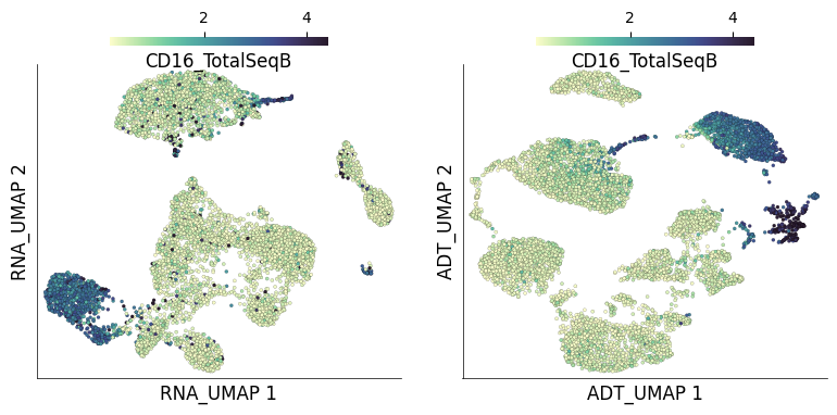
Individual ADT expression can be visualized in both UMAPs easily.
ds.plot_layout(
    layout_key=['RNA_UMAP', 'ADT_UMAP'],
    color_by='CD16_TotalSeqB',
    from_assay='ADT',
    width=4,
    height=4,
    n_columns=2,
    point_size=5
)
time: 3.2 s (started: 2023-05-24 14:50:37 +00:00)
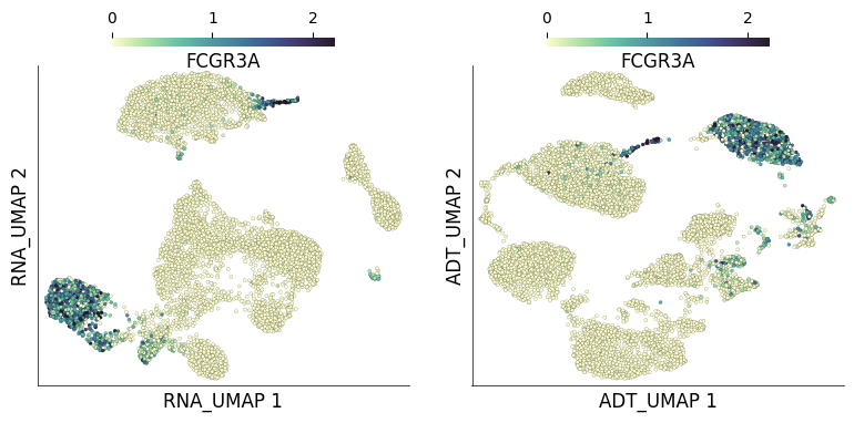
We can also query gene expression and visualize it on both RNA and ADT UMAPs. Here we query gene FCGR3A which codes for CD16:
ds.plot_layout(
    layout_key=['RNA_UMAP', 'ADT_UMAP'],
    color_by='FCGR3A',
    from_assay='RNA',
    width=4,
    height=4,
    n_columns=2,
    point_size=5
)
time: 3.56 s (started: 2023-05-24 14:50:40 +00:00)
6) Integration of modalities#
The KNN graphs created individually for each of the modalities can be merged together to provide an integrated mutimodal view of the data. Scarf takes the latest KNN graphs (continous form edge weight) generated for each of the user chosen modality and merges the edges from each modality. After first round of merging, Scarf performs edge pruning by penalizing those edges more that have lower number of shared nearest neighbors between the connected cells. For each cells edges are pruned until the same number of edges as in individual modalities’ KNN graphs are left.
Here we will integrate the RNA and ADT assays and run UMAP and leiden clustering on the integrated graph.
ds.integrate_assays(
    assays=['RNA', 'ADT'],
    label='RNA+ADT'
)
time: 12.6 s (started: 2023-05-24 14:50:43 +00:00)
integrated_graph parameter in run_umap and run_leiden_clustering allows running these steps on the integrated graph.
ds.run_umap(
    integrated_graph='RNA+ADT',
    n_epochs=500,
    spread=5,
    min_dist=0.5,
    parallel=True
)

ds.run_leiden_clustering(
    integrated_graph='RNA+ADT',
    resolution=1.75
)
time: 1min 16s (started: 2023-05-24 14:50:56 +00:00)
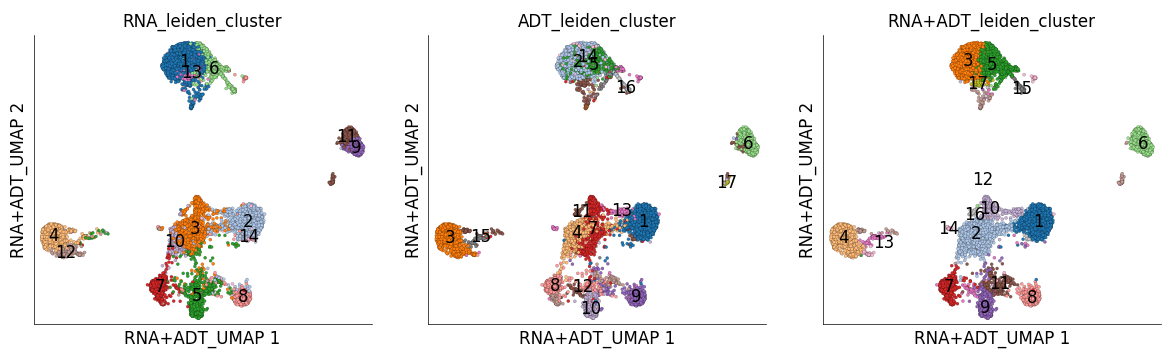
Lets visualize the UMAPs created using the integrated manifolds from the two modalities. Here we label the cells based on their modality specific cluster identity as well as integrated manifold cluster identity
ds.plot_layout(
    layout_key=['RNA+ADT_UMAP'],
    color_by=['RNA_leiden_cluster',
              'ADT_leiden_cluster',
              'RNA+ADT_leiden_cluster'],
    cmap='tab20',
    legend_onside=False,
    point_size=5,
    width=4,
    height=4,
    n_columns=3
)
time: 1.38 s (started: 2023-05-24 14:52:12 +00:00)
ds.cells.columns
['I',
 'ids',
 'names',
 'ADT_UMAP1',
 'ADT_UMAP2',
 'ADT_leiden_cluster',
 'ADT_nCounts',
 'ADT_nFeatures',
 'RNA+ADT_UMAP1',
 'RNA+ADT_UMAP2',
 'RNA+ADT_leiden_cluster',
 'RNA_UMAP1',
 'RNA_UMAP2',
 'RNA_leiden_cluster',
 'RNA_nCounts',
 'RNA_nFeatures',
 'RNA_percentMito',
 'RNA_percentRibo']
time: 6.66 ms (started: 2023-05-24 14:52:13 +00:00)
The UMAP and clustering calculated on the integrated graph are here saved under cell attribute table with prefix RNA+ADT
That is all for this vignette.