Cellular heterogeneity with scRNA-seq#

This tutorial follows one recommended path from a 5K PBMC count matrix to broad cellular populations and marker genes. The dataset is small enough for teaching and has familiar immune-cell structure. It is not evidence for Scarf’s scaling claims; see Scale, memory, and execution for measured resource profiles.

Prerequisites#

Scarf installed with the extra optional dependencies (installation)
Basic familiarity with count matrices

What you will learn#

Convert Cell Ranger H5 to Zarr and open a DataStore
Filter cells without deleting them from the store
Select informative genes and build a neighbourhood graph step by step
Run UMAP and Leiden clustering on that graph
Compare the Leiden result with Scarf’s hierarchical Paris alternative
Rank marker genes per cluster and inspect known immune markers

Dataset#

tenx_5K_pbmc_rnaseq is a public 10x Genomics PBMC dataset distributed through the scarf_docs Cytebase repository.

import numpy as np
import pandas as pd

import scarf

scarf.configure_output(level='WARNING', progress=True)

dataset = scarf.cytebase.connect("scarf_docs").download_dataset(
    'tenx_5K_pbmc_rnaseq',
    destination='scarf_datasets',
)

Downloading bucket files89041311 / 89041311 complete89041311 / 89041311 complete

Downloading bytes89041311 / 89041311 complete89041311 / 89041311 complete

1. Import#

Read the Cell Ranger H5 file, inspect cell and feature counts, then write a Zarr store.

Note

A Zarr “file” is a directory hierarchy on disk, not a single HDF5-style file.

reader = scarf.CrH5Reader(f'{dataset}/data.h5')
reader.nCells, reader.nFeatures

(5025, 33538)

writer = scarf.CrToZarr(
    reader,
    zarr_loc=f'{dataset}/data.zarr',
)
writer.dump()

Writing counts2 / 2 complete2 / 2 complete

Open a DataStore. On first open Scarf streams the count matrix once to compute initialization statistics: per-cell QC columns such as RNA_nCounts and RNA_nFeatures, mito/ribo fractions when gene-name patterns match, and per-feature nCells and dropOuts columns. min_features_per_cell marks cells inactive when they have fewer non-zero features than the threshold. The physical feature column I remains all true; feature filtering is an explicit artifact-producing step.

Opening this store prints a message that the smallest cell count is below the RNA size factor of 1000. It refers to normalization, which is covered in step 3, and the QC filter in step 2 removes those cells.

ds = scarf.DataStore(
    f'{dataset}/data.zarr',
    nthreads=4,
    min_features_per_cell=10
)
ds

Computing RNA initialization statistics1 / 1 complete1 / 1 complete

WARNING: Minimum cell count (502) is lower than size factor multiplier (1000)

DataStore has 5025 (5025) cells with 1 assays: RNA
   Cell metadata:
            'I', 'ids', 'names', 'RNA_percentMito', 'RNA_percentRibo', 
            'RNA_nFeatures', 'RNA_nCounts'
   RNA assay has 33538 features and following metadata:
            'I', 'ids', 'names', 'nCells', 'feature_type', 
            'genome', 'dropOuts'

Active cells, assay feature counts, and the QC column names computed on open.

2. Quality control#

Inspect QC distributions, then set dataset-specific thresholds. Thresholds below are chosen for this PBMC dataset; other datasets need their own cutoffs. Deeper QC options, including auto_filter_cells and doublet detection, are in Quality control across assays.

qc_cols = [
    c for c in (
        'RNA_nCounts', 'RNA_nFeatures', 'RNA_percentMito', 'RNA_percentRibo'
    )
    if c in ds.cells.columns
]
ds.plots.distribution(
    keys=qc_cols,
    kind='violin',
    max_points=2000,
)

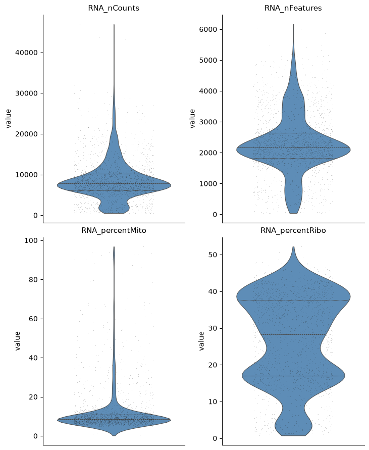
../_images/e9ba125722068740f0eea972cfa4ef8f01340e494692dadaed41789fb65f651b.png

Each violin is one QC metric before filtering; set thresholds from the tails of these distributions.

n_before = int(ds.cells.fetch_all('I').sum())
ds.filter_cells(
    attrs=['RNA_nCounts', 'RNA_nFeatures', 'RNA_percentMito'],
    highs=[15000, 4000, 15],
    lows=[1000, 500, 0]
)
I = ds.cells.fetch_all('I')
print(f'Active cells before filter: {n_before}')
print(f'Active cells after filter: {int(I.sum())}')
print(f'Inactive cells (I=False): {int((~I).sum())}; total in store: {len(I)}')
ds.cells.to_pandas_dataframe(columns=['I'])['I'].value_counts()

Active cells before filter: 5025
Active cells after filter: 3940
Inactive cells (I=False): 1085; total in store: 5025

I
True     3940
False    1085
Name: count, dtype: int64

Note

Filtered cells are marked inactive in the boolean cell key I, not deleted. Most DataStore methods default to cell_key='I'. See Data organization.

ds.plots.distribution(
    keys=qc_cols,
    kind='violin',
    max_points=2000,
    color='coral',
)

../_images/43991bb0a696ddb5977d1432cee5747d24f8e8a6253443694868bccc9e3aa610.png

After filtering, the same metrics are restricted to active cells (I=True).

3. Feature selection#

mark_hvgs ranks genes by corrected variance and marks highly variable genes. It returns an immutable feature selection artifact and publishes the same Boolean values under the plain label hvgs. There is no cell-key prefix.

By default, Scarf excludes common mitochondrial, ribosomal, cell-cycle, HLA/H2, histone, and sex-linked gene-name patterns, together with genes detected in nearly every selected cell. These defaults reduce technical and broadly shared signals in this teaching workflow. Use blacklist="" to keep all names, pass a custom regular expression for a dataset-specific exclusion, or set max_cells=np.inf to disable the ubiquitous-gene filter. The Choosing informative features guide explains the exact patterns and how to compare feature sets.

hvg_ref = ds.mark_hvgs(
    min_cells=20,
    top_n=500,
    min_mean=-3,
    max_mean=2,
    max_var=6,
    show_plot=True,
)
print('Selected genes:', int(ds.RNA.feats.fetch_all('hvgs').sum()))
hvg_ref

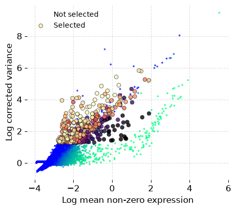
Calculating feature statistics30 / 30 complete30 / 30 complete

../_images/d102679676c3ae4b1f358b3dede5432d5532d66bd7137a13ee2298b43e62324e.png

Selected genes: 498

ArtifactRef(assay='RNA', kind='feature_selection', artifact_id='ac2b9f5f2dc9...')

The selected genes should span the fitted mean-variance trend rather than being concentrated among only the most abundant genes. Very few retained genes or a selection dominated by one gene family warrants inspection before continuing.

4. Normalization#

By default, run_normalization scales each selected cell profile by the sum of its selected features (here the HVGs; renormalize_subset=True), multiplies by ds.RNA.sf, and applies log1p (log_transform=True). Full RNA_nCounts library size is used only when renormalize_subset=False. The default size factor is 1000, and the earlier filter removes cells below that count.

normalized = ds.run_normalization(features=hvg_ref)
status = ds.inspect_artifact(normalized)
opts = status.execution_options or {}
print('Size factor (ds.RNA.sf):', ds.RNA.sf)
print('cell_key:', opts.get('cell_key'))
print('feature selection:', status.inputs['feature_selection'])

Writing data1 / 1 complete1 / 1 complete

Size factor (ds.RNA.sf): 1000
cell_key: I
feature selection: {'type': 'artifact', 'scope': 'assay', 'kind': 'feature_selection', 'artifact_id': 'ac2b9f5f2dc9ecdb5b1064fff7ec92bd87cd31e201960efa4c0b2db68677f2be', 'assay': 'RNA'}

The normalized artifact records both the active cell selection and the hvgs feature selection.

5. PCA#

PCA represents the dominant axes of variation among the selected genes. Fifteen components are sufficient for this controlled PBMC example; the elbow plot shows explained variance flattening after the early components.

ds.run_pca(dims=15, show_elbow_plot=True)

Fitting PCA1 / 1 complete1 / 1 complete

Writing reduced coordinates1 / 1 complete1 / 1 complete

Calculating reduced coordinates1 / 1 complete1 / 1 complete

../_images/6681024fac41fc12a90de6494f961b213add7a57a41a59c164a9fe12d3898c7c.png

ArtifactRef(assay='RNA', kind='reduction', artifact_id='0c9932ea12f6...')

Choosing a component count is a scientific decision on new data. The Choosing dimensionality reductions guide shows how to compare choices.

6. Graph construction#

The remaining steps index the PCA coordinates, find nearby cells, and turn those neighbours into a weighted graph. Downstream layouts and clusters consume this graph rather than the count matrix directly.

ds.build_embedding_initialization()
ds.build_ann_index()
ds.query_neighbors(k=11)
ds.build_connectivity_map()

graph = ds.load_graph()
degrees = graph.getnnz(axis=1)
print(graph.shape, graph.nnz)
print(
    'Degree min / median / max:',
    int(degrees.min()),
    int(np.median(degrees)),
    int(degrees.max()),
)

Loading kmeans coordinates1 / 1 complete1 / 1 complete

Fitting ANN1 / 1 complete1 / 1 complete

Identifying neighbors1 / 1 complete1 / 1 complete

(3940, 3940) 43340
Degree min / median / max: 11 11 11

load_graph returns the result as a sparse cell-by-cell matrix. Shape and nnz confirm the graph covers the active cells; the degree summary checks that neighbourhood sizes stay near the requested k.

7. UMAP#

Run UMAP on the current graph recorded in AssayState. Results are stored as RNA_UMAP1 and RNA_UMAP2.

ds.run_umap(
    n_epochs=250,
    spread=5,
    min_dist=1,
    parallel=True
)

Training UMAP250 / 250 complete250 / 250 complete

ArtifactRef(assay='RNA', kind='embedding', artifact_id='ac51799977d5...')

ds.plots.embedding(layout_key='RNA_UMAP')

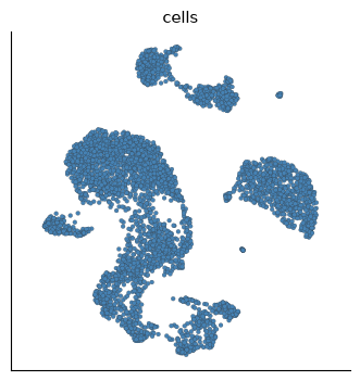
../_images/4c262498abfa207ec5b09739ccc3e51eeaa27156e3ac956d289b9e9a7fb48085.png

Cells are placed by neighbourhood-graph proximity on the UMAP.

ds.plots.embedding(
    layout_key='RNA_UMAP',
    color_by='RNA_nCounts',
)

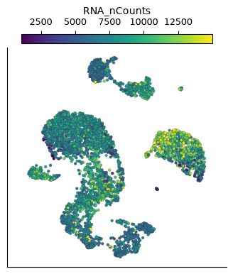
../_images/c200ba56c69dd124e25ab88c1559b068bffaf46cfc826cf8f0eb54ed93262796.png

Library size varies across the embedding; check whether high-count cells dominate one region.

UMAP preserves local neighbourhood evidence but its global distances and empty space are not quantitative measurements. Parameter choice, densMAP, and t-SNE are covered in Choosing dimensionality reductions.

8. Clustering#

Leiden clustering runs on the same neighbourhood graph. This manual call saves labels as RNA_leiden_cluster. ds.pipeline.run() instead writes RNA_leiden_<resolution> columns (for example RNA_leiden_0.5) and copies the selected partition to RNA_clusters.

ds.run_leiden_clustering(resolution=0.5)
ds.cells.to_pandas_dataframe(
    columns=['RNA_leiden_cluster'],
    key='I'
)['RNA_leiden_cluster'].value_counts().sort_index()

RNA_leiden_cluster
    698
     25
    235
   1266
    318
    511
    454
    143
    263
    15
    12
Name: count, dtype: int64

Cluster sizes are worth a look before plotting: a resolution that is too high splits one cell type into several small clusters.

ds.plots.embedding(
    layout_key='RNA_UMAP',
    color_by='RNA_leiden_cluster',
)

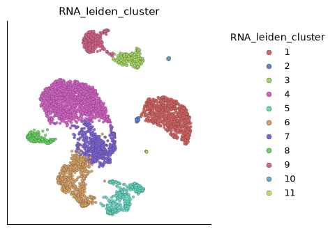
../_images/532f495702a3813e6d7fcff8a18415c93dbb3af7b55a8eba6c93dedbe193ce6c.png

Each colour is a Leiden partition on the same UMAP coordinates.

Paris provides a hierarchical view of the same graph. Its automatic cut is a useful second checkpoint, not a replacement for biological validation.

paris = ds.run_paris_clustering()
ds.cells.to_pandas_dataframe(
    columns=[paris.label_key],
    key='I'
)[paris.label_key].value_counts().sort_index()

RNA_paris_cluster
    721
    245
   1170
    318
    534
    167
    255
    503
     15
    12
Name: count, dtype: int64

ds.plots.embedding(
    layout_key='RNA_UMAP',
    color_by=paris.label_key,
)

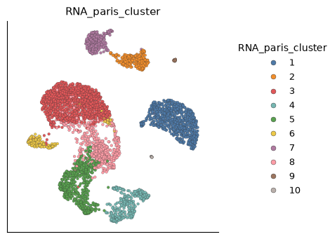
../_images/da9803f22b4d0090d3a5f0c27cee82f98bbe3dce0d9a40397764b6237fdd025e.png

pd.crosstab(
    pd.Series(ds.cells.fetch('RNA_leiden_cluster', key='I'), name='Leiden'),
    pd.Series(ds.cells.fetch(paris.label_key, key='I'), name='Paris'),
)

Paris	1	2	3	4	5	6	7	8	9	10
Leiden
1	696	0	0	0	0	0	2	0	0	0
2	25	0	0	0	0	0	0	0	0	0
3	0	234	0	0	0	0	1	0	0	0
4	0	0	1157	0	0	33	0	76	0	0
5	0	0	0	317	1	0	0	0	0	0
6	0	0	1	1	499	0	0	10	0	0
7	0	0	3	0	34	0	0	417	0	0
8	0	0	9	0	0	134	0	0	0	0
9	0	11	0	0	0	0	252	0	0	0
10	0	0	0	0	0	0	0	0	15	0
11	0	0	0	0	0	0	0	0	0	12

Both partitions should preserve broad monocyte, B-cell, and T-cell structure. The sizes and Leiden×Paris crosstab make that concordance readable before the marker step. Tiny isolated clusters dominated by low-count cells are a reason to revisit QC before interpreting markers. Resolution sweeps, cluster confidence, graph connectivity, and the Paris tree are covered in Choosing and validating clusters.

9. Marker genes#

run_marker_search ranks genes per group. Results include specificity-oriented scores, Mann-Whitney U test p-values (p_value), AUC effect sizes, and within-group Benjamini-Hochberg adjusted values (p_value_adjusted). The adjusted column is a cell-level marker correction for that group, not replicate-aware differential expression. For condition-level DE with full workflows, export counts (see Pseudobulk and differential expression) and use an external tool.

all_features = ds.resolve_features('RNA', 'all_features')
marker_ref = ds.run_marker_search(
    group_key='RNA_leiden_cluster',
    features=all_features,
)

Finding markers2 / 2 complete2 / 2 complete

ds.plots.marker_heatmap(
    marker=marker_ref,
    group_key='RNA_leiden_cluster',
    topn=5,
    figsize=(5, 9)
)

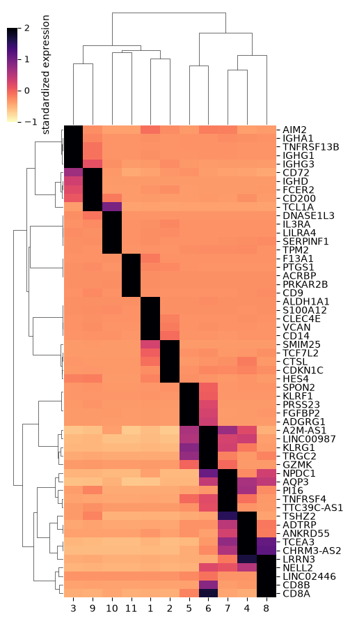
Aggregating marker values per group1 / 1 complete1 / 1 complete

../_images/57a15796bfdbcd709858e729c9a42b9e65ae4ff795b6667ecc245ded3fe48613.png

Rows are top marker genes per cluster; stronger scores mark more cluster-specific genes.

df = ds.get_markers(
    marker=marker_ref,
    group_key='RNA_leiden_cluster',
    group_id='1',
    min_score=-1,
    min_frac_exp=-1
)
df.head()

	group_id	feature_name	feature_index	score	mean	mean_rest	frac_exp	frac_exp_rest	fold_change	auc
0	1	S100A12	1925	0.94637	1.32931	0.00231	0.95559	0.01295	576.70382	0.97670
1	1	VCAN	9167	0.92161	1.48563	0.00465	0.98281	0.03023	319.20089	0.99070
2	1	CD14	9635	0.91601	0.93184	0.00253	0.96991	0.01789	368.28125	0.98420
3	1	ALDH1A1	16188	0.90086	0.12503	0.00019	0.53152	0.00123	665.04820	0.76522
4	1	CLEC4E	20297	0.89682	0.11839	0.00021	0.59742	0.00185	562.32262	0.79802

Rank the same three lineage genes across all Leiden groups before plotting them on the embedding.

markers = ds.get_markers(
    marker=marker_ref,
    group_key='RNA_leiden_cluster',
    group_id=None,
    min_score=-1,
    min_frac_exp=-1,
)
panel = markers[markers['feature_name'].isin(['CD14', 'MS4A1', 'CD3D'])]
panel.sort_values(
    ['feature_name', 'score'], ascending=[True, False]
).groupby('feature_name', sort=False).head(2)

	group_id	feature_name	feature_index	score	mean	mean_rest	frac_exp	frac_exp_rest	fold_change	p_value	auc	p_value_adjusted
2	1	CD14	9635	0.91601	0.93184	0.00253	0.96991	0.01789	368.28125	0.000000e+00	0.98420	0.000000e+00
62101	2	CD14	9635	0.04756	0.05383	0.16789	0.32000	0.18570	0.32061	2.872799e-01	0.54189	1.000000e+00
167765	6	CD3D	18652	0.25896	0.69458	0.33277	0.97847	0.57276	2.08726	9.056661e-87	0.76310	8.437286e-84
201358	7	CD3D	18652	0.20820	0.54457	0.35822	0.97797	0.57946	1.52021	2.830919e-37	0.67888	1.309992e-34
268331	9	MS4A1	17795	0.48917	1.12988	0.07421	0.98859	0.09247	15.22584	0.000000e+00	0.96320	0.000000e+00
67092	3	MS4A1	17795	0.48078	1.09192	0.08459	0.99574	0.09879	12.90776	0.000000e+00	0.96130	0.000000e+00

ds.plots.embedding(
    layout_key='RNA_UMAP',
    color_by=['CD14', 'MS4A1', 'CD3D'],
    n_columns=3,
    sort_values=True,
)

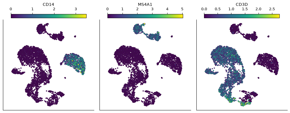
../_images/7f6353e4aaaffd690dfbc453347d693dec16007a9034bfa65e251257d14c5fbb.png

CD14, MS4A1, and CD3D mark monocyte-, B-, and T-cell-like regions when those lineages are present. The lookup above names which Leiden clusters rank each gene highest.

Annotation from markers, known gene panels, and subclustering is covered in Interpreting markers and assigning cell types.

10. Feature imputation#

Graph diffusion is optional and is not part of this default workflow. See Imputation by graph diffusion for a focused comparison of observed and imputed expression, including the limits on interpretation.

Common mistakes and limitations#

Reusing QC thresholds from another dataset without inspecting distributions
Selecting too few genes to represent rare populations, or so many that technical variation dominates
Choosing PCA dimensions or neighbours without checking whether the resulting graph is connected and biologically plausible
Interpreting UMAP distances or empty space as measured biological distances
Treating every extra cluster at a higher resolution as a distinct cell type
Requesting marker tests for groups with fewer than two target or reference cells
Treating marker p_value or within-group p_value_adjusted columns as replicate-aware DE results
Expecting filtered cells to disappear from ds.cells (they remain, with I=False)

Cellular heterogeneity with scRNA-seq

Sections

Cellular heterogeneity with scRNA-seq#

Prerequisites#

What you will learn#

Dataset#

1. Import#

2. Quality control#

3. Feature selection#

4. Normalization#

5. PCA#

6. Graph construction#

7. UMAP#

8. Clustering#

9. Marker genes#

10. Feature imputation#

Common mistakes and limitations#